The Problem of Time in Physics
The
Problem of Time in Physics
The map is not the territory.
(Phillip Darrington, former editor of Wireless World)
Aim and Motivation
It is possible to argue that what is usually being referred to as the Principle of Causality is actually not a principal category, instead it emerges from:
the finite propagation velocity of energy (thus also matter and information);
the quantum fluctuations at the fundamental level, preventing exact repeatability and resulting in the unidirectionallity of events.
Furthermore, it is the complex functioning of the human brain which gives rise to the psychological time and a sense of continuity. Time as a concept, convenient as it may be, is unnecessary, and as a dimension it is also physically inconsistent. Time does not exist.
Disclaimer
Every author of every book or article presenting modern physics in a popular form draws the red line in the colour of his own pet theory. In spite of trying hard to be as objective as possible, this article is no exception. But that is OK as long as the author leaves enough traces to track his line of thought back to the original theoretical works that have made a milestone in the history of science. In this way the reader can make up his own opinion.
Introduction
In the same way as the map is not the territory, a scientific theory is not the natural reality, instead it is always a more or less simplified model of reality. Not because a theory would be incomplete or impossible to complete in principle, but out of necessity. For example, one can never hope to be able to describe the working of, say, a computer by following every single electron, even with the behaviour of every electron well known. Such a task is just too complex, and at a certain level of complexity one wants to switch to some simplifications, approximations, and generalizations of a higher level model in order to finish the required math within the schedule. However, proper modeling requires lots of knowledge of actual phenomena and lots of mathematical skill, so that the accepted model is both simple enough to work with, and complex enough to be faithful to the modeled reality up to the required level of precision.
In physics, processes are often modeled as functions of time, without much thinking about it. Mostly it is a justifiable simplification of no consequence to the result. But as science is advancing, such approach is becoming increasingly unsatisfactory.
Time is commonly regarded as one of the basic physical dimensions, as well as one of the basic units of measure. The human psychological sense of time flow developed on the basis of cosmological changes and general environmental and biological changes influencing our everyday experience. For our ancestors time was originally of a cyclic nature, and only later it was understood as a linear and unidirectional phenomenon. Consequently this sense of “time flow” strongly influenced the development of our language, so that today it is almost impossible to form a sentence in which the notion of time would not be present explicitly or implicitly.
At a first impression the existence of time seems logical, natural, well defined, obvious, and self evident. However, as we start to think about it in a physically and philosophically consistent manner we soon discover that our notion of time is determined too vaguely, and its implementation in physics is rather sloppy, to say the least.
Here we shall skip the usual references to πάντα ρέι (panta rhei, “everything flows”) of Heraclitus, and other ancient Greek philosophers, and come straight to d'Alembert, who in 1754 in his article Dimensions for the Diderot's Encyclopédie wrote:
“Everything that can be measured or expressed in numbers in one way or another can be
thought of as a dimension. A friend of mine thinks that even time might be a dimension.”
To openly express views such as this at the time often meant risking one's own career and good reputation, so it is understandable that d'Alembert cautiously assigned those words to “his friend”; nevertheless, to many of his contemporaries it was perfectly clear that this friend was actually d'Alembert himself. Anyway, it is important to note that this was probably the first explicit historical reference to the possible dimensionality of time.
To Newton, time (as well as space, the cause of gravity, the origin of forces in general) was a given feature of the Universe, on which he distinctly refused to speculate (“Hypotheses non fingo!”), as he concentrated only on the question of how the Universe worked, leaving the “why” deliberately unanswered. In his understanding, time ought to be universal, omnipresent, and absolute, affecting equally (or being obeyed by) each and every object. Yet all forces acting between those objects have been considered instantaneous, since no appreciable amount of aberration could be detected between the line of sight and the direction of gravity of any of the bodies within the Solar system. In spite of motion being treated as an explicit function of time, no force propagation terms are found in the equations of Newton's laws of motion. This later led Laplace to conclude that gravity should be either acting instantaneously, or propagating many orders of magnitude faster than light. The cause for such a conclusion can be traced to Laplace's accounting for only the linear term (v/c), instead of a quadratic term (v2/c2) of the object's velocity v in respect to the light propagation velocity c. Today there is a prevailing expectation that gravity should propagate at the speed of light, though no definite poof has yet been found (only indirect ones), and the debate remains open, see for example the Wikipedia page Speed of Gravity.
With the development of thermodynamics during the XIX century it was argued that the unidirectionality of time arises from entropy, which in a closed system can only increase. Such views were in turn criticized based on the argument that biologic organisms present a typical example of a (local) decrease of entropy. Later, as the structure of the Universe (star planetary system, galaxies, galactic clusters, etc.) became known, there was plenty of evidence of matter self-organization. However, this is hardly a contradiction, since any local decrease of entropy comes at the expense of a general increase.
In the XX century the development of cosmological theories, and with the Big Bang scenario eventually being accepted as an important part of the Standard Model, brought up the question of the beginning of time, as well as why and how it emerges from the fundamental laws of physics. There seems to be a wide consensus that time started together with the Universe, and that before the Big Bang there was no time, thus the term “before” has no meaning.
Minkowski's Spacetime
Our view of the notion of time has changed radically by Einstein's Special (and later General) Theory of Relativity, and the consequent incorporation of time into the spacetime of Minkowski. There is still some confusion today over the actual meaning behind the approach taken by Minkowski, so we shall follow his route in the hope of clarifying the resulting picture. To do this properly we must return to the classical graphical presentation of what we usually refer to as “time dependent” functions, and ponder upon some fairly trivial, but seldom considered expressions.
Consider a classical description of the movement of an object (say, a car traveling on an ordinary city street between two traffic lights), plotted with the time variable t as the abscissa, and the road r(t) as the ordinate, as in Fig.1.
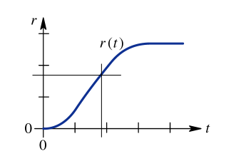
Fig.1:
Graphical representation of the movement of an object.
We usually refer to such a system of coordinates as the Cartesian system (after Cartesius, which was a Latin name of René Descartes). Although Descartes in his La Géométrie never explicitly required that the two axes should be orthogonal, it was exactly this type of graph that eventually got named after him, even if the orthogonal 2D and 3D space has been formally in use from Euclid's Elements onward. The usefulness of the Cartesian coordinate system is owed to the fact that such a representation ensures mutual independence of the two sets of coordinates. For example, in Fig.1, when the object comes to a stop (somewhere in the 4th time interval), its spatial coordinate remains the same, but its temporal coordinate continues to increment. This is in accordance with our everyday experience: as you now sit by your PC reading this text, your spatial coordinates do not change (referred to your surroundings), but you are still aging.
From Fig.1 it is obvious that the car started to accelerate from the origin (0,0) to the first time division, then continued at some constant speed between the first and the second time division, then it decelerated between the second and the third time division, and finally came to stop after the third division. The distance traveled by the car can be represented by a function r(t) = ∫ v(t)dt. This can be differentiated to obtain the instantaneous velocity, v(t) = dr/dt, and the velocity function can be differentiated further to obtain the instantaneous acceleration, a(t) = dv/dt. In the simple case when the car is moving with a constant velocity, the road traveled can be found simply as:
r = vt …....................................................................... (1)
Now comes the funny part! In this last expression, the road r can be considered as a vector quantity, and the velocity v is also a vector (bold letters are used to represent vectors). Obviously, the velocity vector v must point in the same direction as the road vector r, otherwise the car would go off the road and crash. We are thus entitled to ask a “stupid” question:
Is time a vector?
Most of us will be tempted to say of course, time must be a vector. OK, then we can write (1) as the following vector product: r = v × t. But remember that in Fig.1 we have explicitly drawn the time axis orthogonal to the road axis, whilst this vector equation will be mathematically, physically and philosophically correct only if the time vector t is perfectly aligned with the road r. If the time vector t is orthogonal to the road vector r, then the velocity vector v should be orthogonal to both r and t, as required by the vector product operation. But that would be a physical nonsense!
This conflict forces us to conclude that time cannot be a vector quantity, it can only be a scalar quantity, if anything! We are now going to see how Minkowski tried to avoid this conclusion, and made an even greater mess.
Minkowski realized that the type of diagramme as in Fig.1 is inconvenient for the presentation of relativistic phenomena, because the Theory of Relativity and the Lorentz transforms require that the proper time of a moving object is influenced by the object's speed v, normalized to the speed of light c, in the form:
t' = t [1 − (v/c)2 ]−1/2 ........................................................................ (2)
Suppose that in Fig.1 t is measured in seconds [s], and r in meters [m]. Minkowski wanted to put both axes to an equal metric, so he used the speed normalization v/c. In such a presentation the time axis is “geometrized” into ct. The equation of movement (1) then becomes r = (v/c)ct. Because the speed of light c is the highest speed possible, the trajectory (“world line”) of a ray of light would then be plotted as a line tilted at 45°, since in the reference frame of light both axes now have an equal metric. Thus, because of the finite propagation speed of light, Minkowski was able to separate the currently accessible past and future from the currently inaccessible ones.
However pay attention to the awkward fact that by moving at the speed of light, v = c, the proper time t' ceases to change, Δt' = 0, and this occurs not at a vertical line parallel to r, but at the 45° tilted line of the light trajectory. Likewise, because of Equ.(2), one cannot move or a change the speed along a spatial axis without also affecting the rate of time (represented by the slope of the time axis)!
But Minkowski also introduced one more thing. Because the time metric is now equal to the road metric, the time axis must somehow be separated from the spatial dimensions and made independent of the spatial coordinates. Suppose that we rotate our spatial frame of reference so that the road r is coincident with the spatial x axis. In this way all relativistic phenomena occur only along the x axis, leaving the y and z axes unchanged. But now time must be made orthogonal to all spatial axes. Adding a 4th dimension is not a problem in mathematics, but because the three spatial axes are already occupied and we have a geometrized time ct, the only way to do that would be to multiply time by the imaginary unit, making it ict.
How should we understand this? By returning to a 2D world, if we multiply the x axis by −1 we obtain −x, which is the same as the x axis rotated by 180°. Accordingly, a rotation by 90° is achieved by multiplying the x axis by (−1)1/2, which is by definition the imaginary unit i.
Please note that there is nothing “imaginary” in the imaginary axis, it is simply a rotated version of the real axis, so that they have a single common point, zero (the coordinate system origin).
Thus the multiplication by the imaginary unit simply means that we are dealing with a coordinate axis rotated by 90°. This is shown in Fig.2 for a general in case.
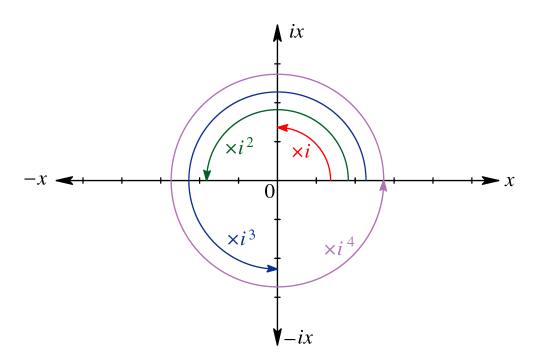
Fig.2:
Rotation by n×90° as the multiplication by in
Now if we would have just two real axes, x and y, and we seek the solution for the equation y = x1/2, the graph will consist of two parts: for x > 0 there will be a parabola in the (x, y) plane, and for x < 0 a parabola in the (x, iy) plane, as shown in Fig.3. The “imaginary” part of the solution simply means that for negative x the solution must be sought in a plane orthogonal to the original (real) plane.
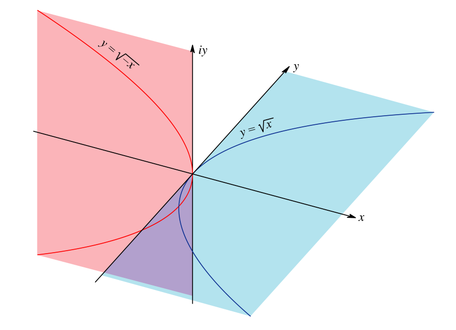
Fig.3:
The complex solution for y = x1/2
Thus with the ict expression Minkowski has geometrized the time axis and rotated it at 90° referred to all other spatial axes. A typical “light-cone” diagramme of Minkowski can be seen in Fig.4.
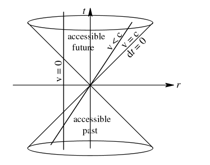
Fig.4:
A typical Minkowski light-cone
In this representation any event which can possibly be perceived from our reference point (the coordinate system origin) must occur within the light-cone, where any velocity v ≤ c. Note that the “rate of time flow” dt goes to zero on the light-cone surface, where the speed v = dr/dt = c. In contrast, in a Cartesian (orthogonal) coordinate system, the dt = 0 should occur on lines which are parallel to the r axis. Therefore such a coordinate system is non-orthogonal, and the axes are not mutually independent! Minkowski's attempt to explain Relativity within an ordinary Cartesian system of coordinates resulted in a non-orthogonal system of coordinates. This is because the time axis is not independent of the rate of change of spatial coordinates, the rate of time “flow” depends on speed, as required by the Theory of Relativity and the Lorentz transforms.
But the non-orthogonality of coordinates is not the only problem in Minkowski's representation.
First, the very dimensionality of time is questionable. The “accessible” past is accessible only from records of past events, one cannot actually go there and revive the moments. And the “accessible” future is accessible only by extrapolation of known states of our near surroundings and known “laws” of physics. What is actually accessible is only the present. As Hawking wrote in his book A Brief History of Time: “If time travel were possible, where are all the tourists from all the future?” (though, to be honest, when I drive towards the Mediterranean coast for my summer vacations, I sometimes wonder...).
Second, the Lorentz transforms require that the rate of time “flow” is affected only along the traveling trajectory, whilst along the coordinates perpendicular to that trajectory no relativistic effects occur! This means that if you choose your coordinate system such that the r axis coincides with, say, the x axis, the rate of time “flow” must be unaffected along the y and z axes. However, when you change your course and move in another direction, the rate of time “flow” should also change in accordance with equation (2) along your new trajectory, and return to the “universal” time along the new perpendicular directions.
Now if time were indeed a “universal” quantity, affecting all objects in the universe, and even being the actual cause of all changes as implied by functional time dependencies like f(t), such an odd behaviour is hard to justify. Moreover, mathematical operations in Minkowski's spacetime appear to occur against the principle of causality. A 4D representation of an event occurring along a 4D diagonal segment
ds = [dx2 + dy2 + dz2 + d(ict)2]1/2 = [dx2 + dy2 + dz2 − c2(dt)2]1/2 ….................... (3)
apparently requires a time inversion, because of i2 = –1. Many physicists feel so uncomfortable with this that, instead of using the diag(+1,+1,+1,−1) as the spacetime unit vector, they rather use diag(−1,−1,−1,+1), and they justify it by saying that one can always choose a system of coordinates such that the three spatial axes are reversed. It is true that time cannot be regarded as a “degree of freedom” of any system, because it is for all our experience unidirectional, whilst the spatial coordinates are bidirectional and can be chosen at will. But such a justification intentionally disregards the cause of the problem, which subsides in the need to separate the time axis from the three spatial axes by a 90° rotation away from each spatial axis, this rotation being represented by the awkward “imaginary” unit i.
Some readers may be puzzled by the fact that the speed of light itself implies the existence of time, as it can be also written as c = dr/dt, just as any other velocity expression; the very existence of movement should therefore imply the existence of time. Well, not necessarily. One way of looking at it is that the dr/dt expression holds only for someone who is trying to measure the speed of light while moving at a very low speed and within a weak gravity field. But if one could accelerate up to the speed of light, moving along a light pulse would not allow him to make any measurement because following Equ. (2) his rate of time “flow” would come to a stop, there would be nothing to measure as no changes would be occurring.
Another way to look at this is by realizing that there is a deeper physical meaning “hidden” beyond the four Maxwell equations within the so called Constitutional Equations for the electric and magnetic fields and the current (transfer of charge) in vacuum:
D = ε0E …................................................................................. (4)
B = μ0H …................................................................................ (5)
J = 0 ……................................................................................. (6)
Here the vector D is the flux density of the electric field with intensity E; B is the flux density of the magnetic field with intensity H. The constant μ0 = 4π×10−7 Vs/Am is the magnetic permeability of free space (vacuum), whilst ε0 ≈ 8.85×10⁻¹² As/Vm is the dielectric permittivity of free space.
Using these equations and solving the electromagnetic wave function we arrive at the following important equations:
c = 1/(ε0μ0)1/2 ……..................................................................... (7)
Z = (μ0/ε0)1/2 ……....................................................................... (8)
Within the SI units the speed of light c and the magnetic permeability μ0 are defined as absolute quantities without any approximation. On the other hand the electromagnetic impedance Z ≈ 367 Ω of vacuum and the dielectric permittivity ε0 are often presented in textbooks as “just happening to have” those particular values. Such a view is wrong, since it is possible to express the permittivity as:
ε0 = 1/(μ0c2) = qe2/(2αhc) …............................................................ (9)
where α = μ0ce2/2h ≈ 1/137 is the fine structure constant, and qe = 1.602×10⁻¹⁹ As is the electron charge. Obviously the electromagnetic properties of vacuum are well defined, and there apparently exists a deep physical connection between the elementary particles (photons, electrons, protons, atoms, ...) and the properties of vacuum.
Consider for example the wave equation often used in quantum electrodynamics and electromagnetic vector calculus:
□φ = −(1/ε0)qeψ*ψ …................................................................ (10)
Here the square symbol □ = (1/c2) ∂2/∂t2 − ∇2 is the d'Alembert operator, the ∇ = 1x∂/∂x + 1y∂/∂y + 1z∂/∂z is the “nabla” operator (unit vectors multiplying the partial derivatives along the appropriate axis), and ψ*ψ is the product of the wave function with its own complex conjugate (effectively the magnitude of the wave function). If in the d'Alembert's operator we write dr/dt instead of c, the time derivatives cancel and the whole wave equation (10) becomes a purely spatial expression.
It is therefore clear that time need not be a necessary ingredient in the definition of fundamental electromagnetic phenomena.
In short, the Minkowski's solution for the graphical representation of relativistic phenomena creates more problems than it solves.
Time in Quantum Theories
Quantum Mechanics was originally developed with time taken as a Newtonian quantity, until Dirac's attempt to introduce the relativistic corrections. His Relativistic Quantum Mechanics became the foundations for the more general Quantum Electrodynamics and then Quantum Field Theory, which narrowed the gaps in some important questions. Today String Theory, Quantum Gravity, Loop Quantum Gravity and other variations are being proposed to finally unify gravity with the quantum world, but discrepancies still exist.
It is not by accident that quantum theories are incompatible with Relativity. Relativity is a classical theory, its results are obtained using Newton's infinitesimal calculus in which dx, dy, dz, and dt can be arbitrary small. Consequently all other quantities, such as energy, can also be arbitrary small. Not so in quantum theories, where energy is quantized in discrete portions, owed to the Planck's constant of minimum action, h. With it, all other quantities should also be quantized at the Planck scale, including space and time. The space quantum should represent a volume proportional to the third power of the Planck's length, which in turn is comparable to the Compton's wavelength of the Planck's mass. Likewise, the Planck's time is the inverse value of the Compton's frequency of the Planck's mass. The numerical values of the Planck's length and time in SI units are given by:
lP = (ħGc−3)1/2 = 1.616×10⁻³⁵ m …................................................................ (11)
tP = (ħGc−5)1/2 = 5.391×10−44 s …................................................................. (12)
where:
ħ = h/2π = 1.055×10⁻³⁴ kg m2 s−2
G = 6.674×10⁻¹¹ m3 kg−1 s−2
c = 299 792 458 m s−1
Another important aspect of quantization is the Heisenberg's Uncertainty Principle, which is in turn a consequence of Heisenberg's non-commutativity of the position-momentum product:
px − xp ≥ ħ/2 ….......................................................................... (13)
This results in a more familiar form of the Uncertainty Principle:
Δp ∙ Δx ≥ ħ/2 .............................................................................. (14)
A similar relation exists between energy and time:
ΔE ∙ Δt ≥ ħ/2 ….......................................................................... (15)
From this relation it is possible to deduce that the minimal time interval is a locally defined quantity, and it depends on the locally available amount of energy:
Δtmin = ħ/2ΔE .............................................................................. (16)
Equation (16) together with (14) leads us to conclude that time is not a universal phenomenon, but a local one, and it actually need not be a physical quantity at all! It seems reasonable to conclude that time does not exist. Instead, it apparently arises from two distinct phenomena:
• the quantum Uncertainty Principle, which prevents any event to be exactly repeated, thus providing the apparent unidirectionality of entropy (the thermodynamical “arrow of time”), and consequently all other events;
• our ability to sense those events and store, retrieve, and compare information about them, thus providing a psychological sense of continuity, further extrapolated as a “flow of time”.
Time Functions Are Not 1:1 Mapped
An important aspect of all physical processes needs to be considered when dealing with time and apparent functions of time. In elementary physics we often consider time functions such that there is a 1:1 mapping between the time axis coordinate and the effective function value at each instant, as in Fig.1. However, no system can actually follow that rule, because energy cannot propagate instantaneously. Instead, real systems behave so that their instantaneous state is a function of not only the current instant, but also all of its past, weighted by the system impulse response. We solve such problems by a mathematical process called the Convolution Integral. The Latin word Convolvere means to fold. The system impulse response f(t) is taken between the time axis origin (t = 0) and some distant time τ, where the impulse response is close enough to zero, and fold it about the origin, so that the function f(t) becomes f(τ – t). Next, we let this folded function slide along the forcing function g(t), and their overlapping parts are multiplied and integrated (summed) for every instant t. The resulting sequence is the response of the system to the forcing function g(t). The animation in Fig.5 shows an example.
Fig.5:
Convolution example
The mathematical expression of the convolution process is:
R(t) = ∫ f(τ − t) g(t) dt …...........….................................................. (17)
Thus it is wrong to say that physical time functions represent instantaneous values of system states in response to instantaneous values of a forcing function. Every system state is a function of not just the current forcing value but also of all the forcing history. However, this is not because of some mysterious “time flow”; instead it is because of the finite propagation velocity of energy within the system and its dissipation in the surroundings.
Time on the Elementary Particle Scale
Considering the discussion above, the question arises: how does time arise on the elementary particle scale?
To be able to properly answer this, we must review the problem of modeling of elementary particles, as well as their interaction with their immediate environment, which also closely relates to some fundamental cosmological questions. Since most readers are not familiar with the quantum world, I find it necessary to cover these issues in a somewhat broader perspective. It is beyond the scope of this article to lead you through all the history of quantum physics. Here I provide only some key points necessary to present a coherent story, possibly leading to a deeper understanding of how time emerges as a consequence of random quantum interactions. The curious reader is encouraged to follow the indicated links at his own pace and pleasure.
Let us examine the most simple example of the electron, e–, and its counterpart the positron, e+ (the signs in the superscript indicate the charge polarity, otherwise their other properties are identical). The electron was identified as a particle in 1897 by J.J. Thomson and his team. The existence of the positron was predicted by Dirac in 1931 and confirmed experimentally in 1932 by Anderson. The electron and the positron represent only one example of matter-antimatter particle pairs in the realm of elementary particles, and amongst many of their well studied properties are the pair creation and annihilation. In these processes a pair of high energy (gamma ray, γ) photons (light quanta, carriers of the electromagnetic interaction) under some favourable conditions is transformed into an electron-positron pair, and vice versa, an electron-positron pair, when coming close enough, readily annihilates into a pair of photons. As an example, the annihilation phenomenon is used in medical diagnostics in Positron Emission Tomography (PET) scans. Symbolically, these processes are written as:
γ + γ ↔ e– + e+ …............................................................... (18)
where the bidirectional arrow indicates that the process is reversible.
So this indicates that matter and antimatter creation from “pure” energy (photons) and back is an ordinary and rather common occurrence in nature! Similar processes (with higher energy photons) occur with all other known particle pairs (mostly inside stars, where both the plasma density and photon density are very high).
Returning to the electron, we consider it as an elementary particle because we have not been able to find any evidence of its internal structure. For all practical purposes it appears to us as a very small, point-like object with a small mass, a unit electrical charge, and an intrinsic angular momentum (spin) with two possible values, ±ħ/2 (Pauli, 1924). This half-unit spin places the electron amongst the fermions, particles that obey the Fermi-Dirac statistics, with the result that within a system not any two identical fermions can be in the same energy state, known as the Pauli Exclusion Principle (in contrast with bosons, particles with integer spin, say, like the photon, which follow the Bose-Einstein statistics, and any number of them can be in the same energy state).
The half-unit spin also means that the electron must make two turns in order to appear the same to the outside world. This is impossible with particles having spherical symmetry, which indicates that the electron does have some kind of internal structure after all, although not such that it can be divided in smaller units. Another problem with a spherically symmetric point-like electron is that it simply cannot sustain the huge Coulomb force resulting from its own charge (because this force is inversely proportional to size and it would diverge to infinity, so the electron would immediately be crushed by its own field at the very moment of its creation), thus it must be of some finite size. It is known that the classical electron radius (based on only the classical electromagnetic theory, ignoring quantum considerations) reveals a figure re = (1/4πε0)(qe2/mec2) ≈ 2.8×10⁻¹⁵ m, where qe is the electron charge and me is the electron mass. An almost identical figure is obtained from other known quantities, the fine structure constant α and the reduced Planck constant: re = αħ/mec. However, observations of single electrons in a Penning trap place an upper limit of the electron radius to ~10−22 m.
This is just one of several discrepancies of our models of elementary particles. This forced us to search for possible alternatives, and for a number of reasons the String Theory is thought to be a viable alternative. One of the strongest arguments in favour of it was the endeavour to unify the Quantum Theory with the General Theory of Relativity. In String Theory one of the basic, naturally occurring forms of particles is a low energy spin 2 particle, very similar to the hypothetical Einstein's graviton, so the very existence of gravity became a rationale for the conceptual correctness of the String Theory.
As the name implies, String Theory objects are tiny strings, both open and closed, with their thickness much smaller than their length, and it is conjectured that various known particles can be modeled by a suitable form and a suitable vibration mode of those strings. For example, a photon might be modeled as an open string, and an electron as a closed string.
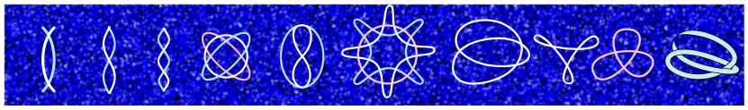
It should be pointed out that the idea of modeling elementary particles with strings and vibration modes is not new. Similar ideas were already discussed by Tait, Maxwell, Thomson, and others. In fact Tait made the first general catalogue of closed strings, based on knots, and developed the Knot Theory, which today is just one aspect of more general Topological studies. Fig.6 shows some examples of those knots. The motif for the interest in knots was in those days to try to model the atoms.
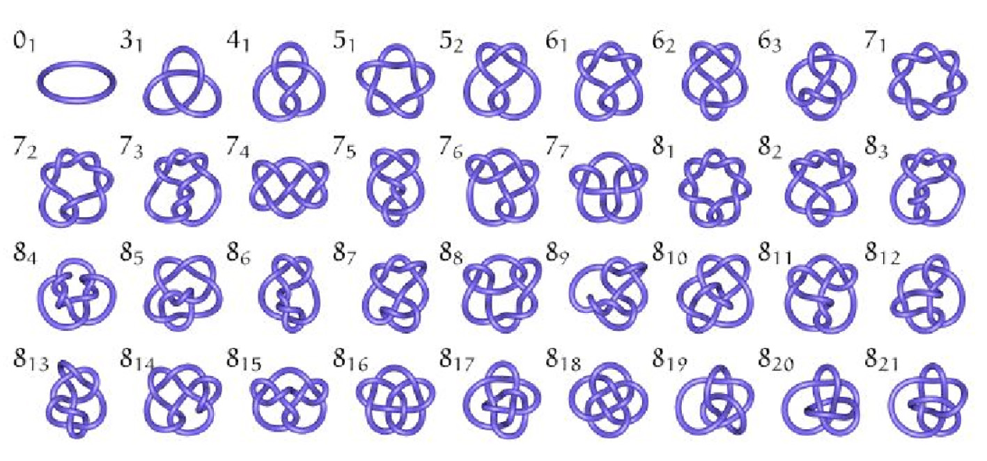
Fig.6:
Examples of Tait knots
Fig.7 shows a transcription of a leter from Maxwell to Tait discussing the subject. Apparently the idea has its roots in the study of water vortex structures by Helmholtz.
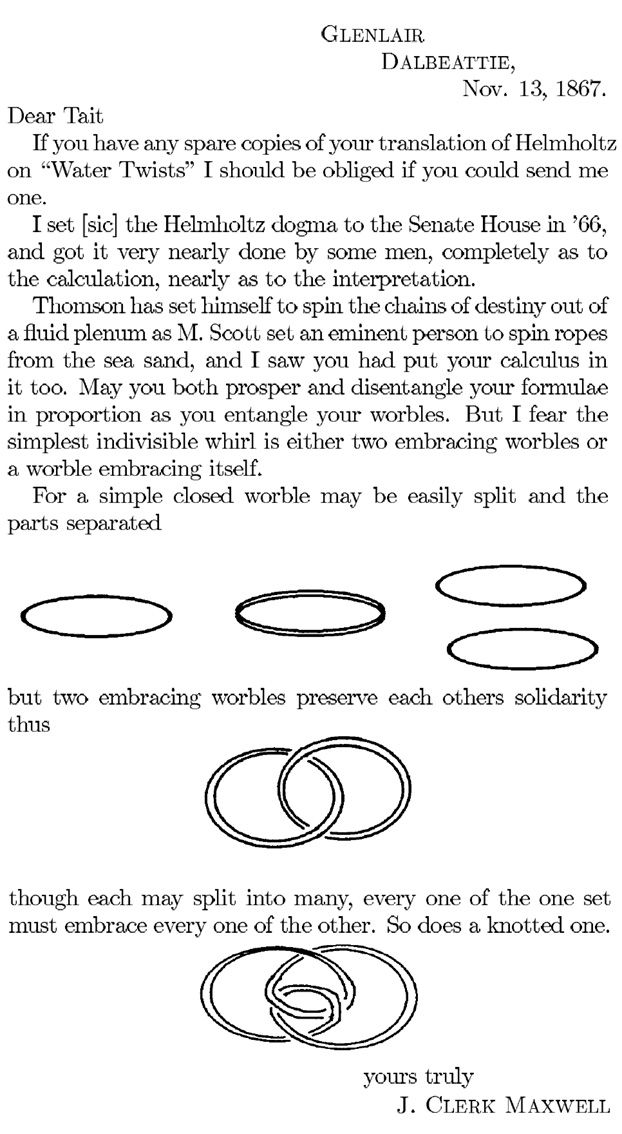
Fig.7:
Maxwell's letter to Tait
What is new in String Theory is that it works in a 10 (or 11) dimensional space, following the dimensionality of the matrix of basic properties of particles. It is not clear why each property must be given its own spatial dimension, probably it is a matter of convenience; for example, it should be possible to express spin in the ordinary 3D space, but that would complicate the equations. There are actually at least 5 different forms of String Theories, which have evolved to include not only strings but also various types of membranes (“branes”). All these theories are thought to be just various simplifications of one General String Theory, yet to be formulated, and possibly to become the “Final Theory”, or the “Theory of Everything”.
In spite of its high promises, today “String Theory is in knots”, as has been ironically observed by Smolin. Besides him, the critics are many, but nevertheless, some ideas which originally emerged within the String Theory are being also examined and accepted within the well established concepts of Quantum Electrodynamics and the Quantum Field Theory. Amongst them, the idea that the electron could be modeled as a torus, or as a Möbius (figure of 8) ribbon are being seriously investigated.
|
|
|
Lately, a number of semi-classical ideas have also been resurrected. Following the work of Thomson (Lord Kelvin) discovering the existence of an absolute lower thermal limit, the works of Planck in 1900 and 1910, and Nernst in 1911, the interpretation of an experiment performed by Einstein and Stern in 1913, see Ref. [1], brought up an interesting realization: what we usually consider to be an empty space (devoid of all matter and all radiation) is not completely empty! In fact, an empty metal box, completely devoid of air and cooled down to almost absolute zero, apparently still contains a certain amount of energy. In calculations, this energy is proportional to (ħ/2)ω for every mode of oscillation (represented by the angular frequency ω) enabled by the system boundaries. This prompted Einstein to coin this phenomenon as the Nullpunktsenergie, the zero-point energy. This was generalized by Nernst, who in 1916 postulated that the vacuum of space is all filled with this zero-point electromagnetic radiation.
If so, why do we not see it with our eyes, just like ordinary light? Certainly, part of that spectrum must also be within the visible range for the human eye. The answer is in Maxwell's superposition theorem, since electromagnetic waves can coexist within the same space, and their waves are linearly combined. Because in a space with large boundaries a large number of wavelengths, frequencies, and phases are possible, every photon can always have a counter phase photon compensating its field. If this radiation is homogeneous and isotropic throughout the Universe, there is no way to detect it, because only energy differences can be observed (thus a closed metal box was needed in the experiment of Einstein and Stern). Fig.9 shows animations of simple two wave superposition cases.
|
|
|
Fig.9: Examples of two wave superposition: a) waves of slightly different frequencies traveling in the same direction produce occasional doubling and cancellation of amplitude; b) waves of equal frequency traveling in opposite directions produce a stationary wave modulated in amplitude.
Later during the XX century several experiments confirmed the existence of vacuum energy directly or indirectly, the most notable was the Casimir effect. Also, the Lamb shift, the Davies-Unruh effect, the van der Waals force, and several others seem to corroborate the hypothesis. The Schrödinger's Zitterbewegung (a kind of oscillatory motion of elementary particles) is thought to be a consequence of this energy. Because for any kind of energy the Heisenberg's Uncertainty Principle applies, the same must be true for the vacuum energy, thus quantum fluctuations in vacuum are expected.
Vacuum energy may seem an odd concept at first, but it is actually required and predicted by both Classical Electrodynamics and Quantum Electrodynamics, as well as other quantum theories. One notable difference between various theories is in the origin of this energy. Classical Electrodynamics threats the problem phenomenologically, the experimental results (Planck's black body radiation, Einstein's and Stern's experiment) force us to modify the equations accordingly, and then the equations receive the theoretical interpretation. In Quantum Electrodynamics the vacuum energy emerges as a result of the Zitterbewegung of all quantum particles, however it is difficult to understand why should there be any energy remaining when all matter and all radiation is removed. In contrast, Stochastic Electrodynamics associates the vacuum energy with the beginning of the Universe, and considers quantum Uncertainty and the Zitterbewegung to be a consequence of vacuum energy influencing every particle.
Recently it was discovered by the observations of distant Supernovae of type Ia that their apparent brightness diminishes with distance more than was expected from a pure Hubble's law of the expansion of the Universe. Based on those observations it was concluded that the expansion of the Universe is accelerating (instead of slowing down under its own gravity, as expected by General Relativity). This acceleration was attributed to a small value of vacuum energy density, and amongst several models the one in which this energy has the same effect as the Einstein's cosmological constant Λ is currently favoured. Because this energy cannot be seen directly, it was labeled as the Dark Energy. From the experimental data this energy density was calculated to be about 10−9 J/m3. This value is rather small, and its effect can be noticed only on very large distances.
However, calculations based on the classical electromagnetic theory (Planck, Einstein-Stern), and calculations based on Quantum Electrodynamics, both give a value of about 10113 J/m3. This is a huge amount of energy, though still finite. In fact, this value stems from the assumption that the electromagnetic interaction is operational and effective down to the Planck scale, with the shortest wavelength (highest frequency, highest energy) of the order of the Planck length (Planck energy).
This discrepancy of 122 orders of magnitude is probably the greatest embarrassment of all physics, and it simply demands to be resolved as soon as possible. There are a few possibilities:
one is that we are making some odd error, because our measurements of cosmic distances are based on the spectral red shift, and we are assigning it all to the expansion of the Universe, whilst it is known that other influences on the spectral shift exist, one is definitely gravitation; if so, vacuum energy is exactly Lorentz invariant, can thus have any value, and has no effect at large scale;
another possibility is that this cosmological Dark Energy does not interact with any other fundamental interaction type but gravity, so it is something currently unknown and out of the Standard Model, thus also different from the ordinary vacuum energy;
a third possibility is that vacuum energy density is not completely proportional to ω3 of the Planck radiation law, so it is not completely Lorentz invariant, and a small part of it is responsible for the observed effect at very large scale;
there is also a possibility that the fundamental constants of nature are not constant, but change with the expansion of the Universe, at least some of them might; although the spectral measurements of distant (high z) galaxies constrain it significantly, they did not rule it out completely;
finally, it is also possible that we live in an oscillating Universe, which has just come out of its minimum phase; then the Friedman solutions to Einstein's field equations do not apply, and the Big Bang model is wrong; in an oscillating universe the contraction phase must of course be driven by gravity, but it is not very clear what force or condition would lead to its expansion, so here again some form of Dark Energy would be needed.
Attempts have been made to recalculate the vacuum energy density based on the assumption of different high frequency cutoffs, ranging from the energy required for the electron-positron pair formation, up to the energy of the most massive particle detected so far, the top quark, thus the top-antitop quark pair.
The reason for this is Equ. (18). If there is enough energy available, randomly the quantum fluctuations may become locally large enough to give birth to a pair of particles more massive than the electron. The animation in Fig.10 shows an example of a superposition of just a small number of waves resulting readily in a high local peak.
Fig.10: Superposition of only a few waves with a particular phase may result in a high local peak.
The particle pair so created annihilates almost immediately, restoring their energy back to their environment. The lifetime of such virtual particle pairs is thought to be governed by the Compton wavelength (for the electron-positron pair that is given by λC = h/mec, so that ωC = 2πc/λC and T = 2π/ωC; numerically this is about 10−22s). Those particles are called “virtual” because they are not detected — if they were detected, the result of the process would be altered, since some of their energy would be lost in the detector, and the particles would appear as “real”.
It is known that if the local field value exceeds the Schwinger limit, ES = me2c3/qeħ ≈ 1.3×10¹⁸ V/m, the vacuum becomes non-linear, superposition is no longer possible, and electron-positron pairs start to appear. As a side thought, it is known that the field strength close to a completely ionized uranium atom is of the order of 1018 V/m, making it understandable why uranium is the last relatively long-term stable element in the Periodic Table.
It is difficult to estimate where exactly should the electromagnetic upper high frequency limit be (in order to allow the integration of the Planck's spectral energy density formula for the ideal black body radiation to return the correct finite value of the spatial vacuum energy density). However, if the production of particle pairs follows a Gaussian statistics, there is some indirect evidence, Ref.[xx], that the peak probability should be close to the pion pair production, so that pion pairs represent the average virtual particle pairs being constantly created and annihilated at a relatively high rate. This rate determines the spatial density of virtual particle pairs in vacuum. Following some reasonable statistical assumptions, based on the average particle energy, lifetime, their coherence length, and the average radiation energy build-up between two adjacent creations and annihilations, it can be calculated that there should be some 5.4×10²⁰ pion pairs at any moment in every cubic meter of space. This may not seem much since there are some 2.5×1025 molecules in a cubic meter of air. However the pop-up rate of virtual particle pairs is huge, about 1042 pairs per cubic meter per second! A brief discussion on the possible value of vacuum energy density is available here.
On the other hand, it is expected by Quantum Field Theory that the vacuum energy should constitute of not only the electromagnetic field, but also fields of other interactions, as well as the Higgs field; this paradigm is gaining acceptance, slowly but steadily. Thus vacuum fluctuations may well be more complex than previously thought.
Be as it may, the main point in all this story is that vacuum quantum fluctuations produce short-lived particle pairs (not single, and not multiple particles, because of the necessity to conserve the total momentum, charge, spin, and all other quantum numbers). Thus those particles must have opposite charge, which during their lifetime causes them to be sensitive to any external fields, behaving as dipoles. In other words, the quantum vacuum is polarizable! This polarizability is what gives the vacuum its electromagnetic properties of magnetic permeability μ0 and dielectric permittivity ε0. A more detailed but sort of “engineering” approach (rather than rigorously theoretical) to the consequences of vacuum polarizabiliy can be found in this article.
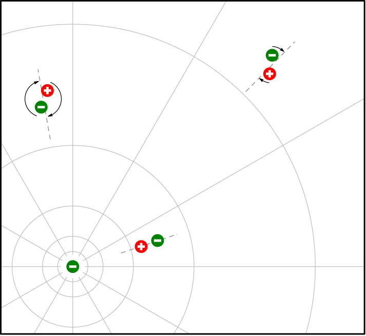
Fig.11:
Schematic display of vacuum polarization: virtual electron-positron
pairs popping up randomly within the field of a real electron; within
its shot life the virtual pair is forced to reorient its position,
the required momentum is influencing the local electron field.
It has also been conjectured that the internal energy of any “real” particle expels the vacuum energy from within the particle, so that its internal energy exactly balances the external vacuum energy, probably owed to the radiation pressure (photon momentum) balance. This balance gives the particles their short or long term stability, not unlike those dolphin-created toroidal air bubbles in water.
Of course the details of all this depend heavily on the particular geometrical and physical particle model employed. Indeed, many models of elementary particles have been devised, some more successful, some less, but so far none of them such that would account for all the known properties of even only the electron, let alone other particles. However, it should be admitted that this area of research is only at the beginning, thus we leave it to theoreticians with experience in topology, and to experimentalists to devise experiments to confirm or reject the proposed models.
What we are interested here is the influence of the surrounding quantum fluctuations on a particle, because those random fluctuations prevent reversible (time-symmetric) billiard-ball physics at the fundamental level. Those fluctuations cause both the Schrödinger's Zitterbewegung and the Heisenberg's Uncertainty, which cause quantum noise, and slight differences in each interaction with other particles, thus ensuring the effective unidirectionality of events, the thermodynamics, the entropy, the apparent macroscopic “flow of time”.
To conclude: the quantum fluctuations set the “deafult” maximum rate of “time flow” at low speed, low gravity, and low energy density conditions. By increasing the speed (or by entering a stronger gravity field), the local symmetry of interaction with vacuum fluctuations in the direction of movement (or the direction of the gravity field) changes, resulting in an apparent slowing of this “time flow” for the object in question, in full accordance with the General Theory of Relativity and the Lorentz transforms.
What Time Is Not
Time is but an illusion of our mind.
Albert Einstein
At the end of our discussion it is appropriate to summarize our views and decide what time is, or should or must be, and what it is not.
Below is a short list of properties and aspects often assigned to time as it is conventionally understood, sorted in relation to its probable (non)existence. Most of the negative attributes have been collected from a variety of articles and theoretical proposals of fundamental physics background, theory unification attempts, and cosmological views.
By no means is this list definitive, nor complete, and neither authoritative in any way. The motivation behind it is to provide a starting point to ponder on the notion of time. Indeed, the readers are encouraged to think of other, new possibilities, as well as impossibilities (which are equally important at this stage of our understanding!).
Time is (regardless of whether it exists or not):
unidirectional (irreversible)
local
instantaneous (non-dimensional)
relative (in the Lorentz/GTR sense), its rate being:
speed dependent
gravity dependent
energy density dependent
maximum rate set universally by quantum fluctuations of the vacuum energy
minimum rate is zero, set by moving at the speed of light, or by a gravity event horizon
If it does exist, time almost certainly isn't:
space-like, but orthogonal to space (in the Minkowski's ict sense)
a dimension (in the same sense as space has dimensions)
a manifestation of extra hidden or tightly wrapped dimensions
an independent variable
a degree of freedom
a vector
a scalar field
a set of coordinates (a “3D movie”)
a coordinate
a “flow” of “something”
a consequence of any and every change
a perpetual “driving force” behind all changes
an abstract “universal numerical order of changes”
a probability amplitude of a change
a period of oscillation (of energy quanta)
an infinitesimal instant (whatever THAT means!)
an ordered sequence of Planck tP intervals
a chaotic attractor (where do people get such funny ideas???)
a unit of interaction
a mutual exchange of “chronons” between interacting elementary particles
a spacetime knot, or a network of knots
If time does not exist, the sensation of time may be arising from:
quantum vacuum fluctuations at the root of Heisenberg's Uncertainty
vacuum electromagnetic properties, conditioning finite energy propagation velocity (c)
human ability to store, retrieve, and compare information, thus forming a mental continuum
rotational degree of freedom (spin?) of elementary particles (???)
Some Important References:
Planck, Max: On the Law of Distribution of Energy in the Normal Spectrum, Annalen der Physik, vol. 4, p. 553 ff (1901), see also: Planck's Law
Einstein, A.: Does the Inertia of a Body Depend upon its Energy-Content? Annalen der Physik, 18:639 (1905)
Einstein, A.; Stern, O. (1913): "Einige Argumente für die Annahme einer molekularen Agitation beim absoluten Nullpunkt". Annalen der Physik 40 (3): 551. Bibcode 1913AnP...345..551E. doi:10.1002/andp.19133450309.
Planck, Max: Uber die begrundung des gesetzes der schwarzen strahlung. Ann. d. Phys. 37, 642, (1912).
Poincaré, H.J.: The End of Matter
Poincaré, H.J.: The Measure of Time
Poincaré, H.J.: The Principles of Mathematical Physics
Poincaré, H.J.: On the Dynamics of the Electron
Sakharov, A.: Vacuum Quantum Fluctuations in Curved Space and the Theory of Gravity
YE Xing-Hao, LIN Qiang: Inhomogeneous Vacuum: An Alternative Interpretation of Curved Spacetime, Chin.Phys.Lett., Vol. 25, No. 5 (2008) 1571 (IOP Science)
Urban, M., Couchot, F., Sarazin, X.: A mechanism giving a finite value to the speed of light, and some experimental consequences, arXiv <http://lanl.arxiv.org/abs/1111.1847v1>, 2011
More on the Physics and the Philosophy of Time
(in no particular order)
<http://en.wikipedia.org/wiki/Time>
<http://en.wikipedia.org/wiki/Philosophy_of_space_and_time#The_flow_of_time>
<http://rationalwiki.org/wiki/Time>
<http://rationalwiki.org/wiki/Timeless_physics>
Anderson, E.: The Problem of Time in Quantum Gravity
Discover Magazine/ Physics & Math / Einstein Newsflash: Time May Not Exist
Edge: The Reality Club:
Kauffman & Smolin: A possible solution to the problem of Time in Quantum Cosmology
Smolin. L: on the Problem of Time
Smolin, L.: The Trouble With Physics: The Rise of String Theory, The Fall of a Science, and What Comes Next, 2008
Harrington, J. (2005): What Kind of a Problem is the Problem of Time?
Quantum Diaries: Alexander, S.: The Problm of Time, Oct.03.2005.
Zeh, H.D.: The Physical Basis of the Direction of Time
Vaessen, R.L.: Time Does Not Exist
Scientific American: Callender, C.: Is Time an Illusion?
The Telegraph: Highfield, R.: The New Theories that are Killing Time
Salles, H.: Does Time Exist?
Journal of Theoretics Vol.3-1 Feb/March 2001 Editorial:
Siepmann, J.P.: Why Time does not Exist
Barbour, J.: The End of Time, Oxford University Press, New York, 2001.
Barbour, J.: The nature of time. arXiv <http://arxiv.org/abs/0903.3489>, 2009.
Woit, P.: Not Even Wrong: The Failure of String Theory and the Search for Unity in Physical Law, 2006
Huggett, N., Vistarini, T., Wüthrich, C.: Time in quantum gravity,
arXiv <http://arxiv.org/abs/1207.1635v1>, 2012
Chappell, J.M., Iannella, N., Iqbal, A., Abbott, D.: A new description of space and time using Clifford multivectors, arXiv <http://arxiv.org/abs/1205.5195v1>, 2012
Balasubramanian, V.: What we don't know about time
arXiv <http://arxiv.org/abs/1107.2897v1>, 2011
Rañada, A.F., Tiemblo, A.: The dynamical nature of time
arXiv <http://lanl.arxiv.org/abs/1106.4400v1>, 2011
Kiefer, C.: Does time exist in quantum gravity?
arXiv <http://arxiv.org/abs/0909.3767>, 2009
Romero, G.E., Pérez, D.: Time and irreversibility in an accelerating universe
arXiv <http://arxiv.org/abs/1105.3626v1>, 2011
Ibison, M.: Electrodynamics with a Future Conformal Horizon
arXiv <http://arxiv.org/abs/1010.3074>, 2010
Bicego, A.: On a probabilistic definition of time
arXiv <http://arxiv.org/abs/1010.2968>, 2010
Carroll, S.: From Eternity to Here: The Quest for the Ultimate Theory of Time, Dutton, 2010
Prati, E.: The Nature of Time: from a Timeless Hamiltonian Framework to Clock Time of Metrology
arXiv <http://lanl.arxiv.org/abs/0907.1707v1>, 2009
Petkov, V.: Time and Reality of Worldtubes
arXiv <http://lanl.arxiv.org/abs/0812.0355v1>, 2008
Goenner, H.F.M.:On the History of Geometrization of Space-time: From Minkowski to Finsler Geometry, arXiv <http://lanl.arxiv.org/abs/0811.4529v1>, 2008
Sidharth, B.G.: Modelling Time, arXiv <http://lanl.arxiv.org/abs/0809.0587v1>, 2008
Wu, Z.C.: The Imaginary Time in the Tunneling Process, arXiv <http://lanl.arxiv.org/abs/0804.0210v1>, 2008
Saniga, M.: Geometry of Time and Dimensionality of Space, arXiv <http://lanl.arxiv.org/abs/physics/0301003>, 2003
Various Discussions:
<http://www.physicsforums.com/showthread.php?t=65439>
<http://www.toequest.com/forum/time-travel/2055-time-does-not-exist.html>
<http://expertscolumn.com/content/exploring-theory-time-does-not-exist>
<http://physics.about.com/od/timetravel/f/doestimeexist.htm>
<http://topdocumentaryfilms.com/through-the-wormhole-does-time-exist/>
<http://gravimotion.info/Does%20time%20exist.htm>
<http://www.psychologytoday.com/blog/biocentrism/201202/does-time-really-exist>
<http://www.newswire.ca/en/story/975685/does-time-exist-perimeter-s-public-lecture-on-june-6>