Tuning your software can make it use hardware capabilities more effectively. Even the fastest machine can render only as fast as the application can drive it. Simple changes in application code can often make a dramatic difference in rendering time. In addition, Silicon Graphics systems let you make trade-offs between image quality and performance for your application.
This chapter looks at tuning graphics applications. Using the following sections, this chapter describes pipeline tuning as a conceptual framework for tuning graphics applications and introduces some other fundamentals of tuning:
Writing high-performance code is usually more complex than just following a set of rules. Most often, it involves making trade-offs between special functions, quality, and performance for a particular application. For more information about the issues you need to consider and for a tuning example, see the following chapters in this book:
After reading these chapters, experiment with the different techniques described to help you decide where to make these trade-offs.
| Note: If optimum performance is crucial, consider using the OpenGL Performer rendering toolkit. See “Maximizing Performance With OpenGL Performer” in Chapter 1. |
This section gives advice on important aspects of OpenGL debugging. Most points apply primarily to graphics programs and may not be obvious to developers who are accustomed to debugging text-based programs.
Here are some general debugging tips for an OpenGL program:
OpenGL never signals errors but simply records them; you must determine whether an error occurred. During the debugging phase, your program should call glGetError() to look for errors frequently (for example, once per redraw) until glGetError() returns GL_NO_ERROR. While this slows down performance somewhat, it helps you debug the program efficiently. You can use ogldebug to automatically call glGetError() after every OpenGL call. See “ogldebug—The OpenGL Debugger” in Chapter 14 for more information on ogldebug.
Use an iterative coding process: add some graphics-related code, build and test to ensure expected results, and repeat as necessary.
Debug the parts of your program in order of complexity: First make sure your geometry is drawing correctly, then add lighting, texturing, and backface culling.
Start debugging in single-buffer mode, then move on to a double-buffered program.
The following are some areas that frequently experience errors:
Be careful with OpenGL enumerated constants that have similar names. For example, glBegin(GL_LINES) works; glBegin(GL_LINE) does not. Using glGetError() can help to detect problems like this (it reports GL_INVALID_ENUM for this specific case).
Use only per-vertex operations in a glBegin()/glEnd() sequence. Within a glBegin()/glEnd() sequence, the only graphics commands that may be used are commands for setting materials, colors, normals, edge flags, texture coordinates, surface parametric coordinates, and vertex coordinates. The use of any other graphics command is invalid. The exact list of allowable commands is given in the man page for glBegin(). Even if other calls appear to work, they are not guaranteed to work in the future and may have severe performance penalties.
Check for matching glPushMatrix() and glPopMatrix() calls.
Check matrix mode state information. Generally, an application should stay in GL_MODELVIEW mode. Odd visual effects can occur if the matrix mode is not right.
This section describes some specific problems frequently encountered by OpenGL users. Note that one generally useful approach is to experiment with an ogldebug trace of the first few frames. See “Creating a Trace File to Discover OpenGL Problems” in Chapter 14. This section covers the following problems:
A common problem encountered in graphics programming is a blank window. If you find your display does not show what you expected, do the following:
To make sure you are bound to the right window, try clearing the image buffers with glClear(). If you cannot clear, you may be bound to the wrong window (or no window at all).
To make sure you are not rendering in the background color, use an unusual color (instead of black) to clear the window with glClear().
To make sure you are not clipping everything inadvertently, temporarily move the near and far clipping planes to extreme distances (such as 0.001 and 1000000.0). (Note that a range like this is totally inappropriate for actual use in a program.)
Try backing up the viewpoint up to see more of the space.
Check the section “Troubleshooting Transformations” in Chapter 3 of the OpenGL Programming Guide, Second Edition.
Remember that glOrtho() and glPerspective() calls multiply onto the current projection matrix; they do not replace it.
If you have a blank window in a double-buffered program, check first that something is displayed when you run the program in single-buffered mode. If yes, make sure you are calling glXSwapBuffers(). If the program is using depth buffering, ensure that the depth buffer is cleared as appropriate. See also “Depth Buffering Problems”.
Check the aspect ratio of the viewing frustrum. Do not set up your program using code like the following:
GLfloat aspect = event.xconfigure.width/event.xconfigure.height
                 /* 0 by integer division */
The following rotation and translation areas might be trouble spots:
Z axis direction
Remember that by default you start by looking down the negative z axis. Unless you move the viewpoint, objects should have negative z coordinates to be visible.
-
Make sure you have translated back to the origin before rotating (unless you intend to rotate about some other point). Rotations are always about the origin of the current coordinate system.
Transformation order
First translating and then rotating an object yields a different result than first rotating and then translating. The order of rotation is also important; for example, R(x), R(y), R(z) is not the same as R(z), R(y), R(x).
When your program uses depth testing, be sure to do the following:
Enable depth testing using glEnable() with a GL_DEPTH_TEST argument; depth testing is off by default. Set the depth function to the desired function, using glDepthFunc(); the default function is GL_LESS.
To guarantee that your program is portable, always ask for a depth buffer explicitly when requesting a visual or framebuffer configuration.
The following two areas might be animation problem areas:
Double buffering
After drawing to the back buffer, make sure you swap buffers with glXSwapBuffers().
Observing the image during drawing
If you have a performance problem and want to see which part of the image takes the longest to draw, use a single-buffered visual. If you do not use resources to control visual selection, call glDrawBuffer() with a GL_FRONT argument before rendering. You can then observe the image as it is drawn. Note that this observation is possible only if the problem is severe. On a fast system, you may not be able to observe the problem.
If you are having lighting problems, try one or more of the followig actions:
Turn off specular shading in the early debugging stages. It is harder to visualize where specular highlights should be than where diffuse highlights should be.
For local light sources, draw lines from the light source to the object you are trying to light to make sure the spatial and directional nature of the light is right.
Make sure you have both GL_LIGHTING enabled and the appropriate GL_LIGHT#'s enabled.
To see whether normals are being scaled and causing lighting problems, enable GL_NORMALIZE. This is particularly important if you call glScale().
Make sure normals are pointing in the right direction.
Make sure the light is actually at the intended position. Positions are affected by the current model-view matrix. Enabling light without calling glLight(GL_POSITION) provides a headlight if called before gluLookAt() and so on.
The following items identify possible problem sources with the X Window system:
OpenGL and the X Window System have different notions of the y direction. OpenGL has the origin (0, 0) in the lower left corner of the window; X has the origin in the upper left corner. If you try to track the mouse but find that the object is moving in the “wrong” direction vertically, this is probably the cause.
Textures and display lists defined in one context are not visible to other contexts unless they explicitly share textures and display lists.
glXUseXFont() creates display lists for characters. The display lists are visible only in contexts that share objects with the context in which they were created.
If you are having problems writing pixels or textures, ensure that the pixel storage mode GL_UNPACK_ALIGNMENT is set to the correct value depending on the type of data. For example:
GLubyte buf[] = {0x9D, ... 0xA7};
         /* a lot of bitmap images are passed as bytes! */
glBitmap(w, h, x, y, 0, 0, buf);
|
The default value for GL_UNPACK_ALIGNMENT is 4. It should be 1 in the preceding case. If this value is not set correctly, the image looks sheared.
The same thing applies to textures.
Traditional software tuning focuses on finding and tuning hot spots, the 10% of the code in which a program spends 90% of its time. Pipeline tuning uses a different approach: it looks for bottlenecks, overloaded stages that are holding up other processes.
At any time, one stage of the pipeline is the bottleneck. Reducing the time spent in the bottleneck is the only way to improve performance. Speeding up operations in other parts of the pipeline has no effect. Conversely, doing work that further narrows the bottleneck or that creates a new bottleneck somewhere else, is the only thing that further degrades performance. If different parts of the hardware are responsible for different parts of the pipeline, the workload can be increased at other parts of the pipeline without degrading performance, as long as that part does not become a new bottleneck. In this way, an application can sometimes be altered to draw a higher-quality image with no performance degradation.
The goal of any program is a balanced pipeline; highest-quality rendering at optimum speed. Different programs stress different parts of the pipeline; therefore, it is important to understand which elements in the graphics pipeline are a program's bottlenecks.
The graphics pipeline in all Silicon Graphics systems consists of three conceptual stages (see Figure 15-1). Depending on the implementation, all parts may be done by the CPU or parts of the pipeline may be done by an accelerator card. The conceptual model is useful in either case: it helps you to understand where your application spends its time.
The following are the three stages of the model:
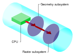
Note that this three-stage model is simpler than the actual hardware implementation in the various models in the Silicon Graphics product line, but it is detailed enough for all but the most subtle tuning tasks.
The amount of work required from the different pipeline stages varies among applications. For example, consider a program that draws a small number of large polygons. Because there are only a few polygons, the pipeline stage that does geometry operations is lightly loaded. Because those few polygons cover many pixels on the screen, the pipeline stage that does rasterization is heavily loaded.
To speed up this program, you must speed up the rasterization stage, either by drawing fewer pixels, or by drawing pixels in a way that takes less time by turning off modes like texturing, blending, or depth buffering. In addition, because spare capacity is available in the per-polygon stage, you can increase the work load at that stage without degrading performance. For example, you can use a more complex lighting model or define geometry elements such that they remain the same size but look more detailed because they are composed of a larger number of polygons.
Note that in a software implementation, all the work is done on the host CPU. As a result, it does not make sense to increase the work in the geometry pipeline if rasterization is the bottleneck: you would increase the work for the CPU and decrease performance.
The basic strategy for isolating bottlenecks is to measure the time it takes to execute a program (or part of a program) and then change the code in ways that do not alter its performance (except by adding or subtracting work at a single point in the graphics pipeline). If changing the amount of work at a given stage of the pipeline does not alter performance noticeably, that stage is not the bottleneck. If there is a noticeable difference in performance, you have found a bottleneck.
CPU bottlenecks
The most common bottleneck occurs when the application program does not feed the graphics subsystem fast enough. Such programs are called CPU-limited.
To see if your application is the bottleneck, remove as much graphics work as possible, while preserving the behavior of the application in terms of the number of instructions executed and the way memory is accessed. Often, changing just a few OpenGL calls is a sufficient test. For example, replacing vertex and normal calls like glVertex3fv() and glNormal3fv() with color subroutine calls like glColor3fv() preserves the CPU behavior while eliminating all drawing and lighting work in the graphics pipeline. If making these changes does not significantly improve performance, then your application has a CPU bottleneck. For more information, see “CPU Tuning: Basics” in Chapter 16.
Geometry bottlenecks
Programs that create bottlenecks in the geometry (per-polygon) stage are called transform-limited. To test for bottlenecks in geometry operations, change the program so that the application code runs at the same speed and the same number of pixels are filled, but the geometry work is reduced. For example, if you are using lighting, call glDisable() with a GL_LIGHTING argument to turn off lighting temporarily. If performance improves, your application has a per-polygon bottleneck. For more information, see “Tuning the Geometry Subsystem” in Chapter 16.
Rasterization bottlenecks
Programs that cause bottlenecks at the rasterization (per-pixel) stage in the pipeline are fill–rate-limited. To test for bottlenecks in rasterization operations, shrink objects or make the window smaller to reduce the number of active pixels. This technique does not work if your program alters its behavior based on the sizes of objects or the size of the window. You can also reduce the work done per pixel by turning off per-pixel operations such as depth buffering, texturing, or alpha blending or by removing clear operations. If any of these experiments speeds up the program, it has a per–pixel bottleneck. For more information, see “Tuning the Raster Subsystem” in Chapter 16.
Usually, the following order of operations is the most expedient:
First determine if your application is CPU-limited using gr_ osview or top and checking whether the CPU usage is near 100%. The gr_osview program (supported only on SGI IRIX systems) also includes statistics that indicate whether the performance bottleneck is in the graphics subsystem or in the host.
Then check whether the application is fill-rate-limited by shrinking the window.
If the application is neither CPU-limited nor fill-rate-limited, you have to prove that it is geometry-limited.
Note that on some systems you can have a bottleneck just in the transport layer between the CPU and the geometry. To test whether that is the case, try sending less data; for example, call glColor3ub() instead of glColor3f().
Many programs draw a variety of things, each of which stresses different parts of the system. Decompose such a program into pieces and time each piece. You can then focus on tuning the slowest pieces. For an example of such a process, see Chapter 17, “Tuning Graphics Applications: Examples”.
Pipeline tuning is described in detail in Chapter 16, “Tuning the Pipeline”. Table 15-1 provides an overview of factors that may limit rendering performance and the stages of the pipeline involved.
Table 15-1. Factors Influencing Performance
Performance Parameter | Pipeline Stage |
|---|---|
Amount of data per polygon | All stages |
Time of application overhead | CPU subsystem (application) |
Transform rate and mode setting for polygon | Geometry subsystem |
Total number of polygons in a frame | Geometry and raster subsystem |
Number of pixels filled | Raster subsystem |
Fill rate for the given mode settings | Raster subsystem |
Time of color and/or depth buffer clear | Raster subsystem |
Timing, or benchmarking, parts of your program is an important part of tuning. It helps you determine which changes to your code have a noticeable effect on the speed of your application.
To achieve performance that is close to the best the hardware can achieve, start following the more general tuning tips provided in this manual. The next step is, however, a rigorous and systematic analysis. This section looks at some important issues regarding benchmarking:
A detailed analysis involves examining what your program is asking the system to do and then calculating how long it should take based on the known performance characteristics of the hardware. Compare this calculation of expected performance with the performance actually observed and continue to apply the tuning techniques until the two match more closely. At this point, you have a detailed accounting of how your program spends its time, and you are in a strong position both to tune further and to make appropriate decisions considering the speed-versus-quality trade-off.
The following parameters determine the performance of most applications:
Consider these guidelines to get accurate timing measurements:
Take measurements on a quiet system.
Verify that minimum activity is taking place on your system while you take timing measurements. Other graphics programs, background processes, and network activity can distort timing results because they use system resources. For example, do not have applications such as top, osview, gr_osview, or Xclock running while you are benchmarking. If possible, turn off network access as well.
Work with local files.
Unless your goal is to time a program that runs on a remote system, make sure that all input and output files, including the file used to log results, are local.
Choose timing trials that are not limited by the clock resolution.
Use a high-resolution clock and make measurements over a period of time that is at least one hundred times the clock resolution. A good rule of thumb is to benchmark something that takes at least two seconds so that the uncertainty contributed by the clock reading is less than one percent of the total error. To measure something that is faster, write a loop in the example program to execute the test code repeatedly.

Note: Loops like this for timing measurements are highly recommended. Be sure to structure your program in a way that facilitates this approach. The function gettimeofday() provides a convenient interface to system clocks with enough resolution to measure graphics performance over several frames. On IRIX systems, call syssgi() with SGI_QUERY_CYCLECNTR for high-resolution timers. If you can repeat the drawing to make a loop that takes ten seconds or so, a stopwatch works fine and you do not need to alter your program to run the test.
-
Verify that the code you are timing behaves identically for each frame of a given timing trial. If the scene changes, the current bottleneck in the graphics pipeline may change, making your timing measurements meaningless. For example, if you are benchmarking the drawing of a rotating airplane, choose a single frame and draw it repeatedly, instead of letting the airplane rotate and taking the benchmark while the animation is running. Once a single frame has been analyzed and tuned, look at frames that stress the graphics pipeline in different ways, analyzing and tuning each frame.
Compare multiple trials.
Run your program multiple times and try to understand variance in the trials. Variance may be due to other programs running, system activity, prior memory placement, or other factors.
Call glFinish() before reading the clock at the start and at the end of the time trial.
Graphics calls can be tricky to benchmark because they do all their work in the graphics pipeline. When a program running on the main CPU issues a graphics command, the command is put into a hardware queue in the graphics subsystem to be processed as soon as the graphics pipeline is ready. The CPU can immediately do other work, including issuing more graphics commands until the queue fills up.
When benchmarking a piece of graphics code, you must include in your measurements the time it takes to process all the work left in the queue after the last graphics call. Call glFinish() at the end of your timing trial just before sampling the clock. Also call glFinish() before sampling the clock and starting the trial to ensure no graphics calls remain in the graphics queue ahead of the process you are timing.
To get accurate numbers, you must perform timing trials in single-buffer mode with no calls to glXSwapBuffers().
Because buffers can be swapped only during a vertical retrace, there is a period between the time a glXSwapBuffers() call is issued and the next vertical retrace when a program may not execute any graphics calls. A program that attempts to issue graphics calls during this period is put to sleep until the next vertical retrace. This distorts the accuracy of the timing measurement.
When making timing measurements, use glFinish() to ensure that all pixels have been drawn before measuring the elapsed time.
Benchmark programs should exercise graphics in a way similar to the actual application. In contrast to the actual application, the benchmark program should perform only graphics operations. Consider using ogldebug to extract representative OpenGL command sequences from the program. See “ogldebug—The OpenGL Debugger” in Chapter 14 for more information.
To benchmark performance for a particular code fragment, follow these steps:
Determine how many polygons are being drawn and estimate how many pixels they cover on the screen. Have your program count the polygons when you read in the database.
To determine the number of pixels filled, start by making a visual estimate. Be sure to include surfaces that are hidden behind other surfaces, and notice whether or not backface elimination is enabled. For greater accuracy, use feedback mode and calculate the actual number of pixels filled.
Determine the transform and fill rates on the target system for the mode settings you are using.
Refer to the product literature for the target system to determine some transform and fill rates. Determine others by writing and running small benchmarks.
Divide the number of polygons drawn by the transform rate to get the time spent on per-polygon operations.
Divide the number of pixels filled by the fill rate to get the time spent on per-pixel operations.
Measure the time spent executing instructions on the CPU.
To determine time spent executing instructions in the CPU, perform the graphics-stubbing experiment described in “Isolating Bottlenecks in Your Application: Overview”.
On high-end systems where the processes are pipelined and happen simultaneously, the largest of the three times calculated in steps 3, 4, and 5 determines the overall performance. On low-end systems, you may have to add the time needed for the different processes to arrive at a good estimate.
Timing analysis takes effort. In practice, it is best to make a quick start by making some assumptions, then refine your understanding as you tune and experiment. Ultimately, you need to experiment with different rendering techniques and perform repeated benchmarks, especially when the unexpected happens.
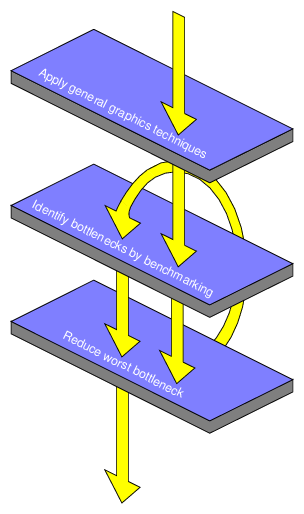
Try some of the suggestions presented in the following chapter on a small program that you understand and use benchmarks to observe the effects. Figure 15-2 shows how you may actually go through the process of benchmarking and reducing bottlenecks several times. This is also demonstrated by the example presented in Chapter 17, “Tuning Graphics Applications: Examples”.
Tuning animation requires attention to some factors not relevant in other types of applications. This section first explores how frame rates determine animation speed and then provides some advice for optimizing an animation's performance.
Smooth animation requires double buffering. In double buffering, one framebuffer holds the current frame, which is scanned out to the monitor by the video hardware, while the rendering hardware is drawing into a second buffer that is not visible. When the new framebuffer is ready to be displayed, the system swaps the buffers. The system must wait until the next vertical retrace period between raster scans to swap the buffers so that each raster scan displays an entire stable frame, rather than parts of two or more frames.
The smoothness of an animation depends on its frame rate. The more frames rendered per second, the smoother the motion appears. The basic elements that contribute to the time to render each individual frame are shown in Table 15-1.
When trying to improve animation speed, consider these points:
A change in the time spent rendering a frame has no visible effect unless it changes the total time to a different integer multiple of the screen refresh time.
Frame rates must be integral multiples of the screen refresh time, which is 16.7 msec (milliseconds) for a 60 Hz monitor. If the draw time for a frame is slightly longer than the time for n raster scans, the system waits for n+1 vertical retraces before swapping buffers and allowing drawing to continue; so, the total frame time is (n+1)*16.7 msec.
If you want an observable performance increase, you must reduce the rendering time enough to take a smaller number of 16.7-msec raster scans.
Alternatively, if performance is acceptable, you can add work without reducing performance, as long as the rendering time does not exceed the current multiple of the raster scan time.
To help monitor timing improvements, turn off double buffering and then benchmark how many frames you can draw. If you do not, it is difficult to know if you are near a 16.7-msec boundary.
The most important aid for optimizing frame rate performance is taking timing measurements in single-buffer mode only. For more detailed information, see “Taking Timing Measurements”.
In addition, follow these guidelines to optimize frame rate performance:
Reduce drawing time to a lower multiple of the screen refresh time (16.7 msec on a 60 Hz monitor).
This is the only way to produce an observable performance increase.
Perform non-graphics computation after glXSwapBuffers().
A program is free to do non-graphics computation during the wait cycle between vertical retraces. Therefore, issue a glXSwapBuffers() call immediately after sending the last graphics call for the current frame, perform computation needed for the next frame, then execute OpenGL calls for the next frame (call glXSwapBuffers(), and so on).
Do non-drawing work after a screen clear.
Clearing a full screen takes time. If you make additional drawing calls immediately after a screen clear, you may fill up the graphics pipeline and force the program to stall. Instead, do some non-drawing work after the clear.