MegaPov version 0.6
This document contains information about MegaPov features that are not part of the official distribution of POV-Ray 3.1. For documentation on the official features, please refer to the official POV-Ray documentation, which can be obtained from www.povray.org.
MegaPov is a cooperative work by members of the POV-Ray community. This is an unofficial version of POV-Ray. Do not ask the POV-Team for help with this. If you need help with a specific patch, contact the author (patch authors are listed in this document, their email address and url are listed in the last chapter). You can get the official version of POV-Ray 3.1 from www.povray.org.
MegaPov features are enabled by using:
#version unofficial MegaPov 0.4; // version number may be different
The new features are disabled by default, and only the official version's syntax will be accepted. The above line of POV code must be included in every include file as well, not just the main POV file.
Once the unofficial features have been enabled, they can be again disabled by using:
#version official 3.1;
This is useful to allow backwards compatibility for the "normal bugfix" and layered textures. Remember, though, that by the normal bugfix and the layered textures bugfix are now disabled by default.
Backwards compatibility is not available for radiosity.
Changing the unofficial version number has no affect on the official language version number. You can also retrieve the unofficial version number using unofficial_version. The unofficial_version variable returns -1 if unofficial features are disabled. Here's an example:
#version 3.1;
#version unofficial MegaPov 0.4;

#declare a= version;
#declare b= unofficial_version;
Here, a would contain the value 3.1, while b would contain the value 0.4.
Author: Mike Hough
syntax:
camera {
  sphere or spherical_camera
  h_angle FLOAT
  v_angle FLOAT
}
The spherical_camera renders spherical views.
The h_angle is the horizontal angle (default 360) and the v_angle is vertical (default 180). Pretty easy.
If you render an image with a 2:1 aspect ratio and map it to a sphere using spherical mapping, it will recreate the scene! Another use is to map it onto an object and if you specify transformations for the object before the texture, say in an animation, it will look like reflections of the environment (sometime called environment mapping for the scanline impaired).
Author: Eric Brown
Bugfixes: Jérôme Grimbert
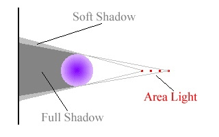
The circular tag has been added to area lights in order to better create circular soft shadows. Ordinary area lights are rectangular and thus project partly rectangular shadows around all objects, including circular objects. By including the circular tag in an area light, the light is stretched and squashed so that it looks like a circle.
Some things to remember:
Circular lights can be ellipses, just give unequal vectors in the scene definition
Rectangular artifacts only show up with large area grids
There is no need to use circular with linear lights or lights which are 2 by 2
The area of a circular light will be 78.5% of a similar size rectangular light (problem of squaring the circle) so increase your vectors accordingly
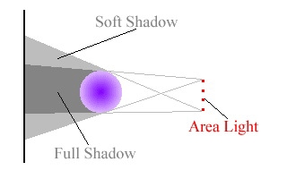
The orient tag has been added to area lights in order to better create soft shadows. Ordinary area lights are 2D (normal lights are 1D); however, if you improperly give the axises to an area light, it can act like a 1D light. By including the orient tag in an area light, the light is oriented so that it acts like a 3D light
Below shows the problem with normal area lights. The axes determine the plane in which the lights are situated. However, this plane can be incorrect for some objects. As such, the soft shadow can be squashed.
The orient tag fixes this by making sure that the plane of the area light is always perpendicular to the point which is being tested for a shadow (see below).
Author: Matthew Corey Brown
syntax
light_source{
  ...
  groups "name1,name2,name3,..."
}
object {
  ...
  light_group "name1"
  no_shadow "name2"
}
media {
  ...
  light_group "!name3"
}
defaults:
light_group "all"
no_shadow "none"
This is to control light interaction of media and objects. There can be a max of 30 user defined Light groups, none and all are pre defined. Groups can be called anything but no spaces and they are delimited by commas with the groups key word. All lights are automatically in the "all" group.
If light_group or no_shadow group contains a ! it is interpreted to mean all lights not in the group that follows the !.
If a light doesn't interact with a media or object then no shadows are cast from that object for that light.
Author: Ronald L. Parker
syntax:
light_source {
  ...
  parallel
  point_at VECTOR
}
Parallel lights shoot rays from the closest point on a plane to the object intersection point. The plane is determined by a perpendicular defined by the light location and the point_at vector.
For normal point lights, point_at must come after parallel.
fade_distance and fade_power use the light location to determine distance for light attenuation.
This will work with all other kinds of light sources, spot, cylinder, point lights, and even area lights.
Author: Nathan Kopp
My latest fun addition to POV is the photon map. The basic goal of this implementation of the photon map is to render true reflective and refractive caustics. The photon map was first introduced by Henrik Wann Jensen <http://www.gk.dtu.dk/home/hwj/>
Photon mapping is a technique which uses a backwards ray-tracing pre-processing step to render refractive and reflective caustics realistically. This means that mirrors can reflect light rays and lenses can focus light.
Photon mapping works by shooting packets of light (photons) from light sources into the scene. The photons are directed towards specific objects. When a photon hits an object after passing through (or bouncing off of) the target object, the ray intersection is stored in memory. This data is later used to estimate the amount of light contributed by reflective and refractive caustics.
I wrote a paper about this for my directed study. The paper is called Simulating Reflective and Refractive Caustics in POV-Ray Using a Photon Map, and you can download it in zipped postscript format at http://nathan.kopp.com/nk_photons.zip (size: about 800 KB).
Current Limitations
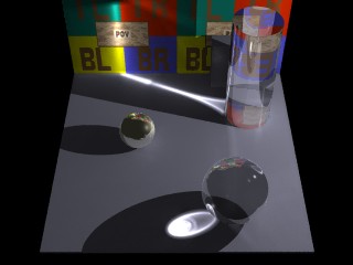 |
This image shows reflective caustics from a sphere and a cylinder. Both use an index of refraction of 1.2. Also visible is a small amount of reflective caustics from the metal sphere, and also from the clear cylinder and sphere. |
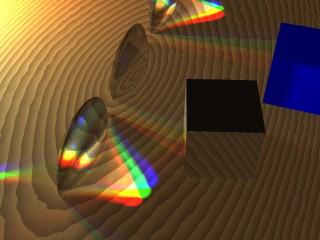 |
Here we have three lenses and three light sources. The middle lens has photon mapping turned off. You can also see some reflective caustics from the brass box (some light reflects and hits the blue box, other light bounces through the nearest lens and is focused in the lower left corner of the image). |
To use photon mapping in your scene, you need to provide POV with two pieces of information. First, you need to specify details about photon gathering and storage. Second, you need to specify which objects receive photons, which lights shoot photons, and how close the photons should be spaced.
To specify photon gathering and storage options you need to add a photons block to the global_settings section of your scene.
Here’s an example:
global_settings{
  photons{
    count 20000
    autostop 0
    jitter .4
  }
}
global_photon_block:
photons {
  spacing <photon_spacing> | count <photons_to_shoot>

  [gather <min_gather>, <max_gather>]
  [global <global_photons_to_shoot>]
  [media <max_steps> [,<factor>]]
  [reflection_blur on|off]
  [jitter <jitter_amount>]
  [max_trace_level <photon_trace_level>]
  [adc_bailout <photon_adc_bailout>]
  [save_file "filename" | load_file "filename"]
  [autostop <autostop_fraction>]
  [expand_thresholds <percent_increase>, <expand_min>]
  [radius <gather_radius>]
  [steps <num_gather_steps>]
}
The number of photons generated can be set using either the spacing or count keywords:
The keyword gather allows you to specify how many photons are gathered at each point during the regular rendering step. The first number (default 20) is the minimum number to gather, while the second number (default 100) is the maximum number to gather. These are good values and you should only use different ones if you know what you’re doing. See the advanced options section for more information.
The keyword global turns on global photons and allows you to specify a count for the number of global photons to shoot.
The keyword media turns on media photons. The parameter max_steps specifies the maximum number of photons to deposit over an interval. The optional parameter factor specifies the difference in media spacing compared to surface spacing. You can increase factor and decrease max_steps if too many photons are being deposited in media.
The keyword reflection_blur allows you to specify whether photons pay attention to reflection blur or not. Usually, blurry caustics can be achieved easily by using fewer photons in the photon map, reducing the need to use true reflection blurring when creating the photon map. Turning on reflection_blur will increase the number of photons if any surfaces use reflection_blur with multiple samples.
The keyword jitter specifies the amount of jitter used in the sampling of light rays in the pre-processing step. The default value is good and usually does not need to be changed.
The keywords max_trace_level and adc_bailout allow you to specify these attributes for the photon-tracing step. If you do not specify these, the values for the primary ray-tracing step will be used.
The keywords save_file and load_file allow you to save and load photon maps. If you load a photon map, no photons will be shot. The photon map file contains all surface (caustic), global, and media photons.
The keyword radius allows you to specify the initial radius used to gather photons. It is suggested that you only specify this if necessary. If you do not specify a gather radius, it will be computed automatically by statistically analyzing the photon map. In some cases you may have to specify it manually, however (which is why the option remains available).
The keywords autostop, steps, and expand_thresholds will be explained later.
To shoot photons at an object, you need to tell POV that the object receives photons. To do this, create a photons { } block within the object. Here is an example:
object{
  MyObject
  photons {
    target
    refraction on
    reflection on
    ignore_photons
  }
}

object_photon_block:
photons{
  [target [<spacing_multiplier>]]
  [refraction on|off]
  [reflection on|off]
  [ignore_photons]
  [pass_through]
}
In this example, the object both reflects and refracts photons. Either of these options could be turned off (by specifying reflection off, for example). By using this, you can have an object with a reflective finish which does not reflect photons for speed and memory reasons.
The keyword target makes this object a target.
The density of the photons can be adjusted by specifying the spacing_multiplier. If, for example, you specify a spacing_multiplier of 0.5, then the spacing for photons hitting this object will be 1/2 of the distance of the spacing for other objects.
Note that this means four times as many surface photons, and eight times as many media photons.
The keyword ignore_photons causes the object to ignore photons. Photons are neither deposited nor gathered on that object.
The keyword pass_through causes photons to pass through the object unaffected on their way to a target object. Once a photon hits the target object, it will ignore the pass_through flag. This is basically a photon version of the no_shadow keyword, with the exception that media within the object will still be affected by the photons (unless that media specifies ignore_photons). New in version 0.5: If you use the no_shadow keyword, the object will be tagged as pass_through automatically. You can then turn off pass_through if necessary by simply using "photons{pass_through off}".
Note: Photons will not be shot at an object unless you specify the target keyword. Simply turning refraction on will not suffice.
light_source{
  MyLight
  photons {
    global
    refraction on
    reflection on
  }
}

light_photon_block :==
photons{
  [global [<spacing_multiplier>]]
  [refraction on|off]
  [reflection on|off]
  [area_light]
}
Sometimes, you want photons to be shot from one light source and not another. In that case, you can turn photons on for an object, but specify "photons {reflection off refraction off}" in the light source’s definition. You can also turn off only reflection or only refraction for any light source.
Light sources can also generate global photons. To enable this feature, put the keyword global in the light source's photon block. The keyword global can be followed by an optional spacing_multiplier float value which adjusts the spacing for global photons emitted from that light source. If, for example, you specify a spacing_multiplier of 0.5, then the spacing for global photons emitted by this light will be 1/2 of the distance of the spacing for other objects. Note that this means four times as many surface photons, and eight times as many media photons (there are currently no global media photons, but eventually that feature will be enabled).
global_settings{
  photons {
    count 10000
    media 100
  }
}
Photons also interact fully with media. This means that volumetric photons are stored in scattering media. This is enabled by using the keyword media within the photons block.
To store photons in media, POV deposits photons as it steps through the media during the photon-tracing phase of the render. It will deposit these photons as it traces caustic photons, so the number of media photons is dependent on the number of caustic photons. As a light ray passes through a section of media, the photons are deposited, separated by approximately the same distance that separates surface photons.
You can specify a factor as a second optional parameter to the media keyword. If, for example, factor is set to 2.0, then photons will be spaced twice as far apart as they would otherwise have been spaced.
Sometimes, however, if a section of media is very large, using these settings could create a large number of photons very fast and overload memory. Therefore, following the media keyword, you must specify the maximum number of photons that are deposited for each ray that travels through each section of media. A setting of 100 will probably work for most
scenes.
You can put ignore_photons into media to make that media ignore photons. Photons will neither be deposited nor gathered in a media that is ignoring them. Photons will also not be gathered nor deposited in non-scattering media. However, if multiple medias exist in the same space, and at least one does not ignore photons and is scattering, then photons will be deposited in that interval and will be gathered for use with all media in that interval.
I made an object with IOR 1.0 and the shadows look weird. Why?
If the borders of your shadows look odd when using photon mapping, don’t be alarmed. This is an unfortunate side-effect of the method. If you increase the density of photons (by decreasing spacing and gather radius) you will notice the problem diminish. I suggest not using photons if your object does not cause much refraction (such as with a window pane or other flat piece of glass or any objects with an IOR very close to 1.0).
My scene takes forever to render. Why?
When POV-Ray builds the photon maps, it continually displays in the status bar the number of photons that have been shot. Is POV-Ray stuck in this step and does it keep shooting lots and lots of photons?
yes
If you are shooting photons at an infinite object (like a plane), then you should expect this. Either be patient or do not shoot photons at infinite objects.
Are you shooting objects at a CSG difference? Sometimes POV-Ray does a bad job creating bounding boxes for these objects. And since photons are shot at the bounding box, you could get bad results. Try manually bounding the object. You can also try the autostop feature (try "autostop 0"). See the docs for more info on autostop.
no
Does your scene have lots of glass (or other clear objects)? Glass is slow and you need to be patient.
My scene has polka dots but renders really quickly. Why?
You should increase the number of photons (or decrease the spacing).
The photons in my scene show up only as small, bright dots. How can I fix this?
The automatic calculation of the gather radius is probably not working correctly, most likely because there are many photons not visible in your scene which are affecting the statistical analysis.
You can fix this by either reducing the number of photons that are in your scene but not visible to the camera (which confuse the auto-computation), or by specifying the initial gather radius manually by using the keyword radius. If you must manually specify a gather radius, it is usually best to also use spacing instead of count, and then set radius and spacing to a 5:1 (radius:spacing) ratio.
Adding photons slowed down my scene a lot, and I see polka dots. Why?
This is usually caused by having both high- and low- density photons in the same scene. The low density ones cause polka dots, while the high density ones slow down the scene. It is usually best if the all photons are on the same order of magnitude for spacing and brightness. Be careful if you are shooting photons objects close to and far from a light source. There is an optional parameter to the target keyword which allows you to adjust the spacing of photons at the target object. You may need to adjust this factor for objects very close to or surrounding the light source.
I added photons, but I don’t see any caustics. Why?
When POV-Ray builds the photon maps, it continually displays in the status bar the number of photons that have been shot. Did it show any photons being shot?
no
If your object has a hole in the middle, do not use the autostop feature (or be very careful with it).
If your object does not have a hole in the middle, you might also try avoiding autostop, or you might want to bound your object manually. As of MegaPov 0.5, you should be able to use "autostop 0" even with objects that have holes in the middle.
Try increasing the number of photons (or decreasing the spacing).
yes
Where any photons stored (the number after "total" in the rendering message as POV shoots photons)?
no
It is possible that the photons are not hitting the target object (because another object is between the light source and the other object). Note that photons ignore the "no_shadow" keyword. You should use photons {pass_through} if you want photons to pass through objects unaffected.
yes
The photons may be diverging more than you expect. They are probably there, but you can’t see them since they are spread out too much
The base of my glass object is really bright. Why?
Use ignore_photons with that object.
Will area lights work with photon mapping?
Photons do work with area lights. However, normally photon mapping ignores all area light options and treats all light sources as point lights. If you would like photon mapping to use your area light options, you must specify the "area_light" keyword within the photons {} block in your light source's code. Doing this will not increase the number of photons shot by the light source, but it might cause regular patterns to show up in the rendered caustics (possibly splotchiness).
What do the stats mean?
In the stats, "photons shot" means how many light rays were shot from the light sources. "photons stored" means how many photons are deposited on surfaces in the scene. If you turn on reflection and refraction, you could get more photons stored than photons shot, since the each ray can get split into two.
Autostop
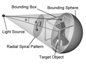 To understand the autostop
option, you need to understand the way photons are shot from light sources. Photons are
shot in a spiral pattern with uniform angular density. Imagine a sphere with a spiral
starting at one of the poles and spiraling out in ever-increasing circles to the equator.
Two angles are involved here. The first, phi, is the how far progress has been made in the
current circle of the spiral. The second, theta, is how far we are from the pole to the
equator. Now, imagine this sphere centered at the light source with the pole where the
spiral starts pointed towards the center of the object receiving photons. Now, photons are
shot out of the light in this spiral pattern.
To understand the autostop
option, you need to understand the way photons are shot from light sources. Photons are
shot in a spiral pattern with uniform angular density. Imagine a sphere with a spiral
starting at one of the poles and spiraling out in ever-increasing circles to the equator.
Two angles are involved here. The first, phi, is the how far progress has been made in the
current circle of the spiral. The second, theta, is how far we are from the pole to the
equator. Now, imagine this sphere centered at the light source with the pole where the
spiral starts pointed towards the center of the object receiving photons. Now, photons are
shot out of the light in this spiral pattern.
Normally, POV does not stop shooting photons until the target object’s entire bounding box has been thoroughly covered. Sometimes, however, an object is much smaller than its bounding box. At these times, we want to stop shooting if we do a complete circle in the spiral without hitting the object. Unfortunately, some objects (such as copper rings), have holes in the middle. Since we start shooting at the middle of the object, the photons just go through the hole in the middle, thus fooling the system into thinking that it is done. To avoid this, the autostop keyword lets you specify how far the system must go before this auto-stopping feature kicks in. The value specified is a fraction of the object's bounding box. Valid values are 0.0 through 1.0 (0% through 100%). POV will continue to shoot photons until the spiral has exceeded this value or the bounding box is completely covered. If a complete circle of photons fails to hit the target object after the spiral has passed the autostop threshold, POV will then stop shooting photons.
The autostop feature will also not kick in until at least one photon has hit the object. This allows you to use "autostop 0" even with objects that have holes in the middle.
Note: If the light source is within the object's bounding box, the photons are shot in all directions from the light source.
Adaptive Search Radius
Many scenes contain some areas with photons packed closely together and some areas where the photons are spaced far apart. This can cause problems, since, for speed reasons, a initial gather radius is used for a range-search of the photon map. Generally, this radius is automatically computed by statistically analyzing the photon map, but it can be manually specified (using the radius keyword) if the statistical analysis produces poor results.
The solution is the adaptive search radius. The gather keyword controls both the minimum and maximum number of photons to be gathered. If the minimum number of photons is not found in the original search radius, we can expand that radius and search again. The steps keyword allows you to specify how many total times to search. The default value for steps is 1.
Using the adaptive search radius correctly can both decrease the amount of time it takes to render the image, and sharpen the borders in the caustic patterns. Usually, using 2 (the default) as the number of steps is good (the initial search plus one expansion). Using too many expansions can slow down the render in areas with no photons, since the system searches, finds nothing, expands the radius, and searches again.
Sometimes this adaptive search technique can create unwanted artifacts at borders (see "Simulating Reflective and Refractive Caustics in POV-Ray Using a Photon Map", Nathan Kopp, 1999). To remove these artifacts, a few thresholds are used, which can be specified by expand_thresholds. For example, if expanding the radius increases the estimated density of photons by too much (threshold is percent_increase, default is 20%, or 0.2), the expanded search is discarded and the old search is used instead. However, if too few photons are gathered in the expanded search (expand_min, default is 40), the new search will be used always, even if it means more than a 20% increase in photon density.
Dispersion
Daren Scott Wilson’s dispersion patch has been incorporated into the photon mapping patch. To use it with photons, you need to specify a color_map in your light source. The color_map will override the light’s color (although you still need to specify the color of the light). The color_map determines the color spectrum for that light source.
I have created a macro, "create_spectrum", which creates a color_map for use with lights. This macro is based on Mr. Wilson’s dispersion patch. See the demo scene "prism.pov" for this macro.
Saving and Loading Photon Maps
It is possible to save and load photon maps to speed up rendering. The photon map itself is view-independent, so if you want to animate a scene that contains photons and you know the photon map will not change during the animation, you can save it on the first frame and then load it for all subsequent frames.
To save the photon map, put the line
save_file "myfile.ph"
into the photons { } block inside the global_settings section.
Loading the photon map is the same, but with load_file instead of save_file. You cannot both load and save a photon map in the POV file. If you load the photon map, it will load all of the photons as well as the range_divider value. No photons will be shot if the map is loaded from a file. All other options (such as gather radius) must still be specified in the POV scene file and are not loaded with the photon map.
Those who have mastered the old syntax for photons may wish to convert old scenes (prior to MegaPov 0.4 and UV-Pov) to the new syntax. This is actually relatively easy.
In each object, simply change the keyword separation to target. The parameter after it remains.
You probably didn't use global photons before, so you do not need to change light sources.
In global settings, either remove radius altogether (it will be automatically computed), or delete the second and third parameters (leaving the first parameter).
If you used a "phd" variable in you scene, you can use the spacing keyword within global_settings. The value specified after spacing will adjust the spacing for all objects that are targets. spacing does not automatically adjust the radius, however.
If you wish to use only one gather step, add the line "steps 1"
inside global_settings.
The steps keyword does the same
thing that the second parameter to radius used to do.
If you used media photons, you'll have to change things a bit. The new syntax is:
media <max_steps> [,<factor>]
You're done
Yes, it is that easy to convert old scenes. And now it is even easier to create new scenes that use photons.
Author: Nathan Kopp
The phong and specular highlighting models available in POV-Ray are alright, but they are quite simplified models. A better model has been developed over the years. This is the Torrance-Sparrow-Blinn-Cook microfacet highlight model.
Blinn highlights (as they will be called) uses statistical methods to simulate microfacets on the surface to produce the highlight. The model uses the fresnel reflectivity equation, which determines reflectivity from the IOR (index of refraction) of the material. For this reason, you must use an interior with an IOR if you want to use blinn highlights.
As with phong and specular, the size blinn highlights can be adjusted. To do this, use the facets keyword. The float value following this keyword specifies the average (r.m.s.) slope of the microfacets. A low value means shallow microfacets, which leads to small highlights. A high value means high slope (very bumpy), which leads to large, soft highlights.
Example:
sphere {
  0.0, 1
  texture {
    pigment {radial frequency 8}
    finish{ blinn 1 facets .2 }
  }
  interior {
    ior 20 // this is a guess for IOR
  }
}
In "ordinary" specular reflection, the reflected ray hits a single point, so there is no dispute as to its color. But many materials have microscopic "bumpiness" that scatters the reflected rays into a cone shape, so the color of a reflected "ray" is the average color of all the points the cone hits.
POV-Ray cannot trace a cone of light, but it CAN take a statistical sampling of it by tracing multiple "jittered" reflected rays.
Normally, when a ray hits a reflective surface, another ray is fired at a matching angle, to find the reflective color. When you specify a blurring amount, a vector is generated whose direction is random and whose length is equal to the blurring factor. This "jittering" vector is added to the reflected ray's normal vector, and the result is normalized because weird things happen if it isn't.
One pitfall you should keep in mind stems from the fact that surface normals always have a length of 1. If you specify a blurring factor greater than one, the reflected ray's direction will be based more on randomness than the direction is "should" go, and it's possible for a ray to be "reflected" THROUGH the surface it's supposed to be bouncing off of.
Since having reflected rays going all over the place will introduce a certain amount of statistical "noise" into your reflections, you have the option of tracing more than one jittered ray for each reflection. The colors found by the rays are averaged, which helps to smooth the reflection. In a texture that already has some noise in it from the pigment, or if you're not using a lot of blurring, 5 or 10 samples should be fine. If you want to make a smooth flat mirror with a lot of blurring you may need upwards of 100 samples per pixel. For preview renders where the reflection doesn't need to be smooth, use 1 sample, since it renders as fast as unblurred reflection.
reflection_blur
Specifies how much blurring to apply. Put this in finish. A vector with this length and a random direction is added to each reflected ray's direction vector, to jitter it.
reflection_samples
Specifies how many samples per pixel to take. It may also be placed in global_settings to change the default without having to specify a whole default texture. Each time a ray hits a reflective surface, this many jittered reflected rays are fired and their colors are averaged. If the finish has a reflection_blur of zero, only one sample will be used regardless of this setting.
Author: Nathan Kopp
One of the features in MegaPov is variable reflection, including realistic Fresnel reflection (see the chapter about 'Variable reflection'). Unfortunately, when this is coupled with constant transmittance, the texture can look unrealistic. This unrealism is caused by the scene breaking the law of conservation of energy. As the amount of light reflected changes, the amount of light transmitted should also change (in a give-and-take relationship).
This can be achieved in MegaPov by adding "conserve_energy" to the object's finish{}. When conserve_energy is enabled, POV will multiply the amount filtered and transmitted by what is left over from reflection (for example, if reflection is 80%, filter/transmit will be multiplied by 20%). This (with a nice granite normal and either media or realistic fade_power) can be used to produce some very realistic water textures.
Many materials tint their reflected light by their surface color. A red Christmas-ornament ball, for example, reflects only red light; you wouldn't expect it to reflect blue. Since the "reflection" keyword takes a color vector, the common "reflection 1" actually gets promoted to "reflection rgb <1, 1, 1>", which would make the ornament reflect green and blue light as well. You'd have to say "reflection Red" to make the ornament reflect correctly.
But what happens if an object's color is different on parts of it? What happens, for example, if you have a Christmas ornament that's red on one side and yellow on the other, with a smooth fade between the two colors? The red side should only reflect red light, but the yellow side should reflect both red and green. (yellow = red + green) Ordinarily, there is no way to accomplish this.
Hence, there is a new feature: metallic reflection. It kind of corresponds to the "metallic" keyword, which affects Phong and specular highlights, but metallic reflection multiplies the reflection color by the pigment color at each point to determine the reflection color for that point. A value of "reflection 1" on a red object will reflect only red light, but the same value on a yellow object reflects yellow light.
reflect_metallic
Put this in finish.
Multiplies the "reflection" color vector by the pigment color at each point
where light is reflected to better model the reflectivity of metallic finishes. Like the
"metallic" keyword, you can specify an
optional float value, which is the amount of influence the reflect_metallic keyword has on the reflected color.
If this number is omitted it defaults to 1.
Note by Nathan Kopp: I have modified this to behave more like the "metallic " keyword, in that it uses the Fresnel equation so that the color of the light is reflected at glancing angles, and the color of the metal is reflected for angles close to the surface’s normal.
Many materials, such as water, ceramic glaze, and linoleum are more reflective when viewed at shallow angles. POV-Ray cannot simulate this, which is a big impediment to making realistic images sometimes.
The only real reflectivity model I know of right now is the Fresnel function, which uses the IOR of a substance to calculate its reflectivity at any given angle. Naturally, it doesn't work for opaque materials, which don't have an IOR.
However, in many cases it isn't the opaque object doing the reflecting; ceramic tiles, for instance, have a thin layer of transparent glaze on the surface, and it is the glaze (which -does- have an IOR) that is reflective.
However, for those "other" materials, I've extended the standard reflectivity function to use not one but TWO reflectivity values. The "maximum" value is the reflectivity observed when the material is viewed at an angle perpendicular to its normal. The "minimum" is the reflectivity observed when the material is viewed "straight down", parallel to is normal. You CAN make the minimum greater than the maximum - it will work, although you'll get results that don't occur in nature. The "falloff" value specifies an exponent for the falloff from maximum to minimum as the angle changes. I don't know for sure what looks most realistic (this isn't a "real" reflectivity model, after all), but a lot of other physical properties seem to have squared functions so I suggest trying that first.
reflection_type
chooses reflectivity function.
The default reflection_type is
zero, which has new features but is backward-compatible. (It uses the 'reflection' keyword.)
A value of 1 selects the Fresnel reflectivity function, which calculates reflectivity
using the finish's IOR. Not useful for opaque textures, but remember that for things like
ceramic tiles, it's the transparent glaze on top of the tile that's doing the reflecting.
Also, Fresnel reflection (reflection_type 1) now pays attention to the reflection_min and reflection_max settings, including colors. The old-style Fresnel reflection always used reflection_min 0.0 and reflection_max 1.0. If reflection_max is zero (or not specified), then MegaPov will default to 0.0 and 1.0 if you use reflection_type 1
reflection_min
sets minimum reflectivity.
For reflection_type 0, this is how reflective the surface will be when viewed from a
direction parallel to its normal.
For reflection_type 1, this will be the minimum reflection.
reflection_max
sets maximum reflectivity.
For reflection_type 0, this is how reflective the surface will be when viewed at a
90-degree angle to its normal.
For reflection_type 1, this will be the maximum reflection.
You can make reflection_min less than reflection_max if you want, although the result is something that doesn't occur in nature.
reflection_falloff
sets falloff exponent in reflection_type 0.
This is the exponent telling how fast the reflectivity will fall off, i.e. linear,
squared, cubed, etc.
reflection
convenience and backward compatibility
This is the old "reflection" keyword. It sets reflection_type to 0, sets both
reflection_min and reflection_max to the value provided, and reflection_falloff to 1.
Authors: Mike Hough (method 2) and Nathan Kopp (method 3)
The new keyword in media, sample_method, can be 1, 2 or 3.
Sample method 1 is the old method of taking samples.
Sample method 2 (invoked by adding the line "method 2" to the
media code) distributes samples evenly along the viewing ray or light ray. The latter can
make things look smoother sometimes.
If you specify a max samples higher than the minimum samples, POV will take additional
samples, but they will be random, just like in method 1. Therefore, I suggest you set the
max samples equal to the minimum samples.
Jitter will cause method 2 to look similar to method 1. It should be followed by a float,
and a value of 1 will stagger the samples in the full range between samples.
Sample method 3 (invoked by adding the line "method 3" to the media code) uses adaptive sampling (similar to adaptive anti-aliasing) which is very much like the sampling method used in POV-Ray 3.0's atmosphere. This code was written from the ground-up to work with media, however.
Adaptive sampling works by taking another sample between two existing samples if there
is too much variance in the original two samples. This leads to fewer samples being taken
in areas where the effect from the media remains constant.
You can specify the anti-aliasing recursion depth using the "aa_level" keyword followed by an integer. You can
specify the anti-aliasing threshold by using the "aa_threshold" followed by a float. The default for "aa_level" is 4 and the default
"aa_threshold" is 0.1.
Jitter also works with method 3.
Sample method 3 ignores the maximum samples value.
It's usually best to only use one interval with method 3. Too many intervals can lead to artifacts, and POV will create more intervals if it needs them.
syntax
media {
  method 2
  jitter
}
Have you ever had POV stop half-way through a render with a "Too few sampling intervals" error? Well, this made me mad on a few occasions (media renders take a long time without having to re-start in the middle). So, if UVPov determines that you need more intervals than you specify (due to spotlights), it will create more for you automatically. So, I suggest always using one interval with method 3.
Author: Lummox JR, July 1999 (beta 0.91)
The isoblob combines the traits of a blob and an isosurface, allowing blob-like components to be specified with user-supplied density functions. The result isn't *perfect*, and nowhere near as good-looking as a regular blob is where simple shapes are involved, but it's not half-bad.
This is the complete isoblob patch, including the function-normal patch it may rely on for more detailed surface normals.
isoblob {
  threshold <THRESHOLD> // similar to blob threshold, not to isosurface
  [accuracy <ACCURACY>]
  [max_trace <MAX_TRACE>] // maximum intersections per interval -- default is quite high
  [normal [on | off]] // Accurate normal calculation -- default is "off", using old method.
  // The function-normal patch makes this keyword available to the
  // isosurface and parametric primitives as well
  // Functions
  // <x, y, z> -- coordinates in component space
  // <r, s, t> -- coordinates in isoblob space
  // Functions should generally return a value from 0 to 1.
  function { ... } // function 1 -- at least one is required
  [function { ... } ...] // functions 2 and up
  // Components
  // Strength is multiplied by the density function to yield true density, just as in blobs
  // Function numbers start at 1, and go in order of definition.
  // Spherical bounding shape
  // Translated so that component space is centered at <0,0,0>
  sphere {
    <CENTER>, <RADIUS>, [strength] <STRENGTH>
    [function] <FUNCTION NUMBER>
    // Insert any other blob-component modifiers here.
  }
  // Cylindrical bounding shape
  // Transformed so that component space is centered around axis from
  // <0, 0, 0> to <0, 0, length>
  cylinder {
    <END1>, <END2>, <RADIUS>, [strength] <STRENGTH>
    [function] <FUNCTION NUMBER>
    // Insert any other blob-component modifiers here.
  }
}
New functions / values allowed for isosurfaces, media, etc.:
Apply accurate normal calculation to isoblobs by using the "normal" keyword (outside of a texture). This can be followed by on/off, true/false, 1/0, etc. The default is to use close approximation, the original method of choice for isosurfaces and parametrics.
Rendering time seems comparable between ordinary calculation and accurate. The more accurate normal calculation may cause a very slight slowdown, but in most cases the difference should be hard to notice.
Any of these functions that are encountered have their normals "fudged" in the same way a normal would otherwise be found for the main function -- by close approximation. There's no point in going through the accurate-normal process in these cases unless accuracy is an overriding concern.
atan2 () doesn't return a proper normal. Anyone with the brains to fix this is welcome to try; I wash my hands of it. I've tried literally everything I could think of, usually at least twice. (The NORMAL_ macros in f_func.c are pretty straightforward; the calculus used is harder).
Many isoblobs may render faster with accurate normals, because of the overhead of transforming x,y,z into component space six times with the close-approximation method.
Q: What is an isoblob?
A: An isoblob is a combination of an isosurface and a blob. An ordinary blob is a combination of shapes with different densities. An isosurface, a primitive type which exists in the Superpatch, can define its surface by a function. The isoblob takes the blob concept and modifies it, so that the density of each component is specified by a function, and thus things like random noise can be included in the density function. Density functions can be defined a lot more specifically and accurately, and with much more flexibility. Plus, more complex shapes are possible than with either a blob or an isosurface alone.
Q: What are the advantages of an isoblob?
A:
Greater flexibility than a blob. A blob can only do two specific types of shapes. Even with heavy modification, it could do few more. Toruses cannot be used in a blob, nor can more complicated functions. A simple box is beyond the capability of a modified blob primitive.
Greater complexity than an isosurface. Even if density functions were added together directly to be combined in a single function, that one function would be overly complicated. By transforming a component's coordinates, its density function can be simplified. And for larger objects with many components, a single function would be too inadequate (and slow) to define the whole thing, even if the function could be made big enough.
Better speed than several isosurface functions. If multiple isosurfaces interacted by adding density values like a blob, the result would be very slow to calculate. In ordinary blobs, the shapes only interact in a few small regions where they overlap. It is easier to calculate density values only where their density could be greater than zero. Thus the ability to set a bounding shape for each component is a great advantage in speed.
Q: What are the disadvantages of an isoblob?
A:
Slower than a blob. A blob is a fine-tuned shape, designed to break things up into small intervals where the shape can be treated like a quartic. It's many times faster than trying to solve for the surface of a function.
Slower than an isosurface. An isosurface uses only a single function, whereas an isoblob breaks up solutions into different intervals where a ray intersects bounding shapes, just like a blob.
Fewer options for finding solutions than an isosurface. An isosurface has the sign value, different methods for solving, etc. The isoblob uses only method 1, assumes a sign of -1 (because the functions are for density values), etc.
Q: Why are the components called "sphere" and "cylinder"?
A: The sphere and cylinder keywords are used to define the bounding shape of each component. A spherical component centered at <5,6,7> with radius 3 will have x, y, and z with a distance of up to 3 units from the origin; the component is then translated to <5,6,7>. (Its <r,s,t> values are centered around <5,6,7>, not the origin.) Similarly, a cylindrical component has x, y, and z values from <0,0,0> to <0,0,length>, length being the length of the cylinder from end to end, and its x and y values stay within the cylinder's radius.
Q: What are the r, s, and t values and how do I use them?
A: <r,s,t> is a vector representing a point in isoblob space, whereas <x,y,z> is the point in component space. Each component has its <x,y,z> values transformed so that all spheres are centered at the origin and all cylinders begin at the origin. However, it is often useful to know where a point will fall after the component has been scaled, rotated, translated, etc. into its final position (within the isoblob, not within the world). Think of <x,y,z> as being the component's personal set of coordinates, and <r,s,t> as the isoblob's. (Note that since components are meant to overlap, it's quite possible for the same <r,s,t> point to have different sets of corresponding <x,y,z> values, one set for each component.
Q: What are some common density functions to use?
A: These are some common density functions, ranging from 0 to 1. Remember that components can be scaled so that different components use the same density function. Squaring a density function will cause more curving where different components meet; if you do this to every density function, be sure to square the threshold also. It is also a good idea to include max(...,0) to avoid negative densities.
Sphere max( 1-sqrt(sqr(x)+sqr(y)+sqr(z))/radius ,0)
Cylinder max( 1-(sqr(x)+sqr(y))/radius ,0)
Box (<x,y,z> from -1 to 1)max( 1-max(max(abs(x),abs(y)),abs(z)) ,0)
Cone (point at z=height) max( 1-z/height-sqrt(sqr(x)+sqr(y))/base_radius ,0)
Torus (around z axis) max( 1-sqrt( sqr( sqrt(sqr(x)+sqr(y))-major_radius )
+sqr(z) )/minor_radius ,0)
Paraboloid (tip at z=height)max( 1-z/height-(sqr(x)+sqr(y))/base_radius ,0)
Helix (one rotation) max( 1-sqrt( sqr(x-major_radius*cos(z*2*pi/height))
+ sqr(y-major_radius*sin(z*2*pi/height) )/minor_radius ,0)
Old blob-style density functions
Blob Sphere sqr(max( 1-sqr((sqr(x)+sqr(y)+sqr(z))/radius) ,0))
Blob Cylinder sqr(max( 1-sqr((sqr(x)+sqr(y))/radius) ,0))
(Ordinary blob cylindrical components have hemisphere end-caps,
which are not included in this function. To accurately simulate an
ordinary blob, you'll need to include the hemispheres manually.)
Blob Base Hemisphere if(z,0, sqr(max( 1-sqr((sqr(x)+sqr(y)+sqr(z))/radius) ,0)))
Blob Apex Hemisphere (translated to end of cylinder) if(z, sqr(max( 1-sqr((sqr(x)
+sqr(y)+sqr(z))/radius) ,0)) ,0)
Author: R. Suzuki
THERE IS NO MANUAL AVAILABLE FOR THE ISOSURFACE PATCH. What follows are tids and bits collected from internet. You will have to read this and look at the examples, then try a few things and see what happens.
Description: With the isosurface patch, you can make iso-surfaces and parametric surfaces for various 3D functions.
You can specify the function both with f(x,y,z) in POV files, and with the name of the functions.
The iso-surface can be used as a solid CSG shape type.
Syntax of "isosurface" object
isosurface {
  function { f1(x, y, z) [ | or & ] f2(x, y, z) .... }
  or function { "functionname", <P0, P1, ..., Pn > }
  // P0, P1,..., Pn are parameters for functionname(x,y,z)
  // function (x, y, z) < 0 : inside for solid shapes.
  contained_by { box {<VECTOR>, <VECTOR> } }  // container shape
  or contained_by { sphere {<VECTOR>, FLOAT_VALUE } }
  [ accuracy FLOAT_VALUE ]
  [ max_trace INTEGER_VALUE [or all_intersections] ]
  [ threshold FLOAT_VALUE ]
  [ sign -1 ] // or 1
  [ max_gradient FLOAT_VALUE]
  [ eval ] // evaluates max_gradient value
  [ method 1 ] // or 2
  [ normal [on | off]] // Accurate normal calculation -- default is "off", using old method.
  [ open ] // clips the isosurface with the contained_by shape
  .....
}
Note: method 2 requires max_gradient value (default max_gradient is 1.1).
The simplest example is:
isosurface { function "sphere", <1> }
The 'function' keyword specifies the potential function you want to see. In this case, it is the "sphere" function which will give you a unit sphere when the parameter is <1>. This can be scaled, rotated and translated.
For an overview of possible built-in function keywords, see further on.
To reduce calculation time, "isosurface" searches the equipotential surface in a finite container region (sphere or box). You can change this region using the "contained_by" keyword with a box or sphere
Note: contained_by {} must be specified or an error message will be given.
isosurface {
  function { "sphere", <6> }
  contained_by { box { <-5, -5, -5>, <5, 5, 5> } }
}
If there is a cross section with the container, "open" allows you to remove the surface on the containing object. On the other hand, if you use "contained_by" without "open", you will see the surface of the container. If you want to use isosurfaces with CSG operations, do not use "open" (and you may have to use "max_trace" in some cases).
[default THRESHOLD_VALUE = 0.0 ]
The potential function of "sphere" is f(x, y, z) = P0 - sqrt(x*x+y*y+z*z)
By default, POV-Ray searches the equipotential surface of f=0. You can change this value using the "threshold" keyword. Then POV-Ray looks for the point where the value of the function equals to the THRESHOLD_VALUE.
isosurface {
  function { "sphere", <1> }
  threshold 0.3
}
In the case of this example, the radius of the sphere is 0.7.
[default = 1 ]
The "sign" keyword specifies which region is inside or outside.
"sign 1": f(x, y, z) -THRESHOLD_VALUE <0 inside
"sign -1": f(x, y, z) -THRESHOLD_VALUE <0 outside
[default MAX_TRACE = 1 ]
This is either an integer or the keyword all_intersections and it specifies the number of intersections to be found with the object. Unless you’re using the object in a CSG, 1 is usually sufficient.
"isosurface" can be used in CSG (CONSTRUCTIVE SOLID GEOMETRY) shapes since "isosurface" is a solid finite primitive. Thus you can use "union", "intersection", "difference", and "merge". By default, "isosurface" routinely searches only the first surface which the ray intersects. However, in the case of "intersection" and "difference", POV-Ray must find not only the first surface but also the other surfaces. For instance, the following gives us an improper shape.
difference {
  sphere { <-0.7, 0, 0.4>, 1 }
  isosurface {
    function { "sphere", <1> }
    translate <0.7, 0, 0>
  }
}
In order to see a proper shape, you must add the "max_trace" keyword.
difference {
  sphere { <-0.7, 0, 0.4>, 1}
  isosurface {
    function { "sphere", <1> }
    max_trace 2
    translate <0.7, 0, 0>
  }
}
[default MAX_GRADIENT = 1.1 ]
The "isosurface" finding routine can find the first intersecting point between a ray and the equipotential surface of any continuous functions if the maximum gradient of the function is known. By default, however, POV-Ray assumes the maximum to be 1. Thus, when the real maximum gradient of the function is 1,
e.g. f= P0-(x*x+y*y+z*z), it will work well.
In the case that the real maximum gradient is much lower than 1, POV-Ray can produce the shape properly but the rendering time will be long. If the maximum gradient is much higher than 1, POV-Ray cannot find intersecting points and you will see an improper shape. In these cases, you should specify the maximum gradient value using the "max_gradient" keyword.
If you do not know the max_gradient of the function, you can see the maximum gradient value in the final statistics message if you add the eval option. If the max_gradient value of the final render is greater than that of the POV file, you should change the max_gradient value.
If you set the eval option without the max_gradient keyword, POV-Ray will try to estimate maximum gradient semi-automatically using results of neighboring pixels. However, this is not a perfect method and sometimes you have to use fixed max_gradient or additional parameters for the eval option.
Since the initial max_gradient estimation value is 1, estimation could work well when the real maximum gradient is around 1 (usually, from 0.5 to ~5). If the real maximum gradient is far from 1, the estimation will not work well. In this case, you should add optional three parameters to eval option.
eval <V1, V2, V3> // where V1, V2, V3 are float values.
The first parameter, V1, is the initial estimation value instead of 1. This means the minimum max_gradient value in the estimation process is V1. The second parameter is the over-estimation parameter (V2 should be 1 or greater than 1) and the third parameter is an attenuation parameter (V3 should be 1 or less than 1). Default is <1, 1.2, 0.99>. If you see an improper shape and want to change the default, you should change (increase) V1 at first.
[ default ACCURACY = 0.001 ]
This value is used to determine how accurate the solution must be before POV stops looking. The smaller the better, but smaller values are slower too.
As "isosurface" finding is a kind of iteration method, you can specify the accuracy of the intersecting point using the "accuracy" keyword to optimize the rendering speed. The default "accuracy" value is 0.001. The higher value (float) will give us faster speed but lower quality. For example,
isosurface {
  function { "torus", <0.85, 0.15> }
  contained_by { box { <-1,-0.15,-1>, <1, 0.15, 1> } }
  accuracy ACCURACY
}
Recursive subdivision method. The equipotential-surface finding in POViso patch is based on a recursive subdivision method as following.
POV-Ray calculates the potential values at the two points (d1 and d2, where d1<d2: the distance from the initial point of the ray).
If there is a possibility (possibility is calculated with a testing function T(f(d1),f(d2), MAX_GRADIENT)) of existence of the equipotential-surface between 'd1' and 'd2', POV-Ray calculates potential value at another point 'd3' on the ray between the two point 'd1' and 'd2'.
If there is a possibility between 'd1' and 'd3', POV-Ray calculates another point 'd4' between 'd1' and 'd3'.
If there is no possibility between 'd1' and 'd3', POV-Ray looks for another point 'd4' between 'd3' and 'd2'.
These calculation (1-4) will be done recursively until (dn-dn')<"ACCURACY".
This POV-Ray version provides two isosurface finding methods. Both methods are based on recursive subdivision. In default, "method 1" is used for parsing functions and "method 2" is used for the functions specified by the name.
Generally, POV-Ray automatically selects the method and the user does not need to specify this keyword.
Author: Lummox JR
Apply accurate normal calculation to isosurfaces and parametrics by using the "normal" keyword (outside of a texture). This can be followed by on/off, true/false, 1/0, etc. The default is to use close approximation, the original method of choice for isosurfaces and parametrics.
Rendering time seems comparable between ordinary calculation and accurate. The more accurate normal calculation may cause a very slight slowdown, but in most cases the difference should be hard to notice.
Anything with a built-in function (Sphere, Helix, etc.) or a pigment function, or anything with noise3d (), should probably use ordinary normal calculation ("normal off") vs. accurate normal if speed is important.
Any of these functions that are encountered have their normals "fudged" in the same way a normal would otherwise be found for the main function -- by close approximation. There's no point in going through the accurate-normal process in these cases unless accuracy is an overriding concern.
atan2 () doesn't return a proper normal. Anyone with the brains to fix this is welcome to try; I wash my hands of it. I've tried literally everything I could think of, usually at least twice. (The NORMAL_ macros in f_func.c are pretty straightforward; the calculus used is harder).
Parametrics may benefit most, speedwise, from a more accurate normal calculation. Depending on the functions used, there may (potentially) even be a minor increase in speed.
Several useful functions are provided in this patch (if known, nr of required parameters and what they control are given):
Added by: Matthew Corey Brown e-mail: <mcb@xenoarch.com>
Manual by: David Sharp e-mail: <dsharp@interport.net>
syntax
function {"ridgedmf", <P0, P1, P2, P3, P4> }ridgedMF(x,0,z) <P0,P1,P2,P3,P4> ("ridged multifractal") can be used to create multifractal height fields and patterns. The algorithm was invented by Ken Musgrave (and others) to simulate natural forms, especially landscapes. 'Multifractal' refers to their characteristic of having a fractal dimension which varies with altitude. They are built from summing noise of a number of frequencies. The ridgedMF parameters <P0, P1, P2, P3, P4> determine how many, and which frequencies are to be summed, and how the different frequencies are weighted in the sum.
An advantage to using these instead of a height_field{} from an image (a number of height field programs output multifractal types of images) is that the ridgedMF function domain extends arbitrarily far in the and z directions so huge landscapes can be made without losing resolution or having to tile a height field.
The function parameters <P0, P1, P2, P3, P4>
(The names given to these parameters refer to the procedure used to generate the function's values and the names don't seem to apply very directly to the resulting images.)
P0 = 'H' is the negative of the exponent of the basis noise frequencies used in building these functions (each frequency f's amplitude is weighted by the factor f - H). In landscapes, and most natural forms, the amplitude of high frequency contributions are usually less than the lower frequencies. When H is 1, the fractalization is relatively smooth ("1/f noise"). As H nears 0, the high frequencies contribute equally with low frequencies (as in "white noise").
P1 = 'Lacunarity' is the multiplier used to get from one 'octave' to the next in the 'fractalization'. This parameter affects the size of the frequency gaps in the pattern. Make this greater than 1.0
P2 = 'Octaves' is the number of different frequencies added to the fractal. Each 'Octave' frequency is the previous one multiplied by 'Lacunarity', so that using a large number of octaves can get into very high frequencies very quickly. (Normally, the really high frequencies contribute little, and will just waste your computing resources.)
P3 = 'Offset' gives a fractal whose fractal dimension changes from altitude to altitude (this is what makes these 'multifractals'). The high frequencies at low altitudes are more damped than at higher altitudes. so that lower altitudes are smoother than higher areas. As Offset increases, the fractal dimension becomes more homogeneous with height.
(Try starting with Offset approximately 1.0).P4 = 'Gain' weights the successive contributions to the accumulated fractal result to make creases stick up as ridges.
Author: David Sharp
syntax:
function {"heteroMF", <H, L, Octs, Offset, T> }heteroMF(x,0,z) <P0,P1,P2,P3,P4> ("hetero multifractal") makes multifractal height fields and patterns of '1/f' noise. 'Multifractal' refers to their characteristic of having a fractal dimension which varies with altitude. Built from summing noise of a number of frequencies, the heteroMF parameters <P0, P1, P2, P3, P4> determine how many, and which frequencies are to be summed.
An advantage to using these instead of a height_field{} from an image (a number of height field programs output multifractal types of images) is that the heteroMF function domain extends arbitrarily far in the and z directions so huge landscapes can be made without losing resolution or having to tile a height field.
The function parameters <P0, P1, P2, P3, P4>
P0 ='H' is the negative of the exponent of the basis noise frequencies used in building these functions (each frequency f's amplitude is weighted by the factor f - H). In landscapes, and many natural forms, the amplitude of high frequency contributions are usually less than the lower frequencies. When H is 1, the fractalization is relatively smooth ("1/f noise"). As H nears 0, the high frequencies contribute equally with low frequencies as in "white noise".
P1 ='Lacunarity' is the multiplier used to get from one 'octave' to the next. This parameter affects the size of the frequency gaps in the pattern. Make this greater than 1.0
P2 ='Octaves' is the number of different frequencies added to the fractal. Each 'Octave' frequency is the previous one multiplied by 'Lacunarity', so that using a large number of octaves can get into very high frequencies very quickly.
P3 ='Offset' is the 'base altitude' (sea level) used for the heterogeneous scaling.
P4 ='T' scales the 'heterogeneity' of the fractal. T=0 gives 'straight 1/f' (no heterogeneous scaling). T=1 suppresses higher frequencies at lower altitudes.
syntax:
function {"hex_x",<0>}function {"hex_y",<0>}The parameter <0> is needed, even if it is only a 'dummy'.
Creates a hexagon pattern. See hex.pov and hex_2.pov in the demo folder for examples.
Build in functions coming from the 'i_algbr' library (+ <nr of parameters needed>).
Build in functions coming from the 'i_nfunc' library.
Build in functions coming from the 'i_dat3d' library.
Manual by: David Sharp
Normally, isosurfaces use a formula to find the values of the isosurface function at the various points in space. On the other hand, one might want to render data for which there is no simple formula, like temperature at different points in a room or data from a CAT scan. In this case, you can make an isosurface from an array of data using the i_dat3d library functions. These are basically the same as the 'formula' isosurfaces, except that the values of the function are given only at discrete 'sample points' and are read from a file or array (rather than calculated from a formula). The values for the function at points in space between sample points are interpolated from the given data. Once declared, they can be combined with other defined isosurface functions in the 'usual' ways. The i_dat3d library functions currently available are:
Functions of the 'i_dat3d' library:
- "data_2D_1" <P0>: a 'height field' over the x-z plane. Points between data points are linearly interpolated (first order). The y sample parameter is ignored.
- "data_2D_3" <P0>: like data_2D_1, but the function values between sample points comes from a cubic interpolation (3rd order), and so the surface is usually smoother.
- "data_3D_1" <P0>: a 3D isolevel surface. Points between data points are linearly interpolated (1st order).
- "data_3D_3" <P0>: like data_3d_1, but the function values between sample points comes from a cubic interpolation (3rd order).
- "odd_sphere" <P0,P1,P2>: This adds data_3d_3 to a sphere.
odd_sphere=P2*sqrt(x*x+y*y+z*z)-P1+data_3D_3
"i_dat3d" calculates (1st or 3rd order) interpolated values from a 3D (or 2D) density distribution data. The distribution data should be specified by the file name in pov file, and will be loaded in the initialize routine.
Example i_dat3d function declaration
#declare MyDataFunction =
function{"data_3D_1", <1> library "i_dat3d","MyData.DAT", <32,32,16,0>}
The "data_3D_1" names which of the i_dat3d library functions to use.
The parameter vector <P0> scales the data.
library "i_dat3d" tells MegaPov that this function requires special initialization. That is, it must read a data file; in this example it would read data from the file "MyData.DAT".
The final vector <32,32,16,0> contains the parameters for the i_dat3d library. : <L0,L1,L2,L3>
- L0 = number of samples in the x direction
- L1 = number of samples in the y direction
- L2 = number of samples in the z direction
In the above example (<32,32,16,0>), the data_3d_1 function 'expects' to find 32*32*16 values in the file "MyData.Dat" arranged as 16 z-planes, each of which is made of 32 y-rows, each row being values at 32 points parallel to 'x'.- L3 tells how the data in the file is formatted:
- 0: text (as could be written out using POV scene language #fwrite()
- 1: 1 byte binary integers
- 2: 2 byte binary integers
- 3: 4 byte binary integers
- 4: 4 byte binary floats
- 5: .DF3 file (POV density file format), but ignore the DF3 file's header sample parameters.
- 6: .DF3 (POV density file format), get the sample parameters (Nx, Ny, Nz) from the DF3 file's header and just ignore the sample parameters found in the library parameter vector <Nx,Ny,Nz,6>
When the data comes from a POV array, the 'L3' library parameter is unnecessary / ignored.
Using a file as the data source, the file must exist before the function is declared. You can also use a POV array as the 'data source'. In this case, you would replace the name of the data file with the name of a predeclared and initialized array of numerical values. Using arrays, function values can be computed in POV scene language using #macros and complex means that would be impossible or impractical from a normal isosurface function formula.
Example declaration of i_dat3d function with an array as data source
#declare MyDataArray=array[32][32][16]
// needs some routine to fill the array with data
#declare MyDataFunction =
function{ "data_3D_1",<1> library "i_dat3d", MyDataArray, <32,32,16>}
Keywords:
z , accuracy, max_gradient, max_trace, func, function, no_eval, eval, lib_name, library, func_id, implicit, r, s, ln, cub, noise3d, all_intersections, func_xy, parametric, isosurface, method, close, sign, int_f, max_grad, precompute, last, contained_by
Functions and operators available:
Two iso-surface finding methods are provided. Both methods are based on recursive subdivision.
In default, "method 1", written by D.Skarda & T.Bily, is used for parsing functions and "method 2", written by R. Suzuki, is used for the functions specified by the name.
Generally, "method 2" is faster than "method 1" for internal functions but it requires information on the maximum gradient of the 3D function.
You can see various examples on
http://www.etl.go.jp/etl/linac/public/rsuzuki/e/povray/iso/
http://atrey.karlin.mff.cuni.cz/~0rfelyus/povray.html
for a beginners tutorial, check out
http://members.aol.com/stbenge/
In addition to the standard mathematical functions, you may use the new pigment function:
syntax:
function { pigment { ... } }
This function will return a value based on the red and green values of the color at the specified point in the pigment. Red is the most significant and green is the least. This is in case you want to use height_field files that use the red and green components. Otherwise just use gray scale colors in your pigment.
This won't work with slope based patterns. You can use them but you'll always get a constant value when its looked up.
parametric {
  function x (u,v) , y (u,v) , z (u,v)
  <u1,v1>, <u2,v2>
  <x1,y1,z1>, <x2,y2,z2>
  [accuracy ACCURACY]
  [precompute DEPTH, VarList]
}
<u1,v1>, <u2,v2>: boundaries to be computed in (u,v) space.
<x1,y1,z1>, <x2,y2,z2>: bounding box of the function in real space.
Accuracy: float value. This value is used to determine how accurate the solution must be before POV stops looking. The smaller the better, but smaller values are slower too.
precompute can speedup rendering of parametric surfaces. It simply divides parametric surfaces into small ones (2^depth) and precomputes ranges of the variables(x,y,z) which you specify after depth. Be careful! High values of depth can produce arrays greater than amount of your RAM.
Example:
parametric {
  function
  u*v*sin (24*v),
  v,
  u*v*cos (24*v)
  <0,0>, <1,1>
  <-1.5,-1.5,-1.5>, <1.5,1.5,1.5>
  accuracy 0.001
  precompute 15, [x, z] // precompute in y does not gain
  // any speed in this case
}
If you declare a parametric surface with the precompute keyword and then use it twice, all arrays are in memory only once.
Author: Nathan Kopp
Triangle mesh objects (mesh and mesh2) can now be used in CSG objects such as difference and intersect, because they do have a defined 'inside.' This will only work for well-behaved meshes, which are completely closed volumes. If meshes have any holes in them, this might work, but the results are not guaranteed.
To determine if a point is inside a triangle mesh, POV-Ray shoots a ray from the point in some arbitrary direction (the default is <1, 0, 0>). If this vector intersects an odd number of triangles, the point is inside the mesh. If it intersects an even number of triangles, the point is outside of the mesh. You can specify the direction of this vector. For example, to use +z as the direction, you would add the following line to the triangle mesh description (following all other mesh data, but before the object modifiers).
inside_vector <0, 0, 1>
This change does not have any effect on unions of triangles... these will still be always hollow.
Author: Nathan Kopp
The new mesh syntax is designed for use in conversion from other file formats. This format was developed by Nathan Kopp and Thomas Baier.
mesh2 {
  vertex_vectors {
    number_of_vertices,
    <vertex1>, <vertex2>, ...
  }
  normal_vectors {
    number_of_normals,
    <normal1>, <normal2>, ...
  }
  uv_vectors {
    number_of_uv_vectors,
    <uv_vect1>, <uv_vect2>, ...
  }
  texture_list {
    number_of_textures,
    texture { Texture1 },
    texture { Texture2 }, ...
  }
  face_indices {
    number_of_faces,
    <index_a, index_b, index_c> [,texture_index [, texture_index, texture_index]],
    <index_d, index_e, index_f> [,texture_index [, texture_index, texture_index]],
    ...
  }
  normal_indices {
    number_of_faces,
    <index_a, index_b, index_c>,
    <index_d, index_e, index_f>,
    ...
  }
  uv_indices {
    number_of_faces,
    <index_a, index_b, index_c>,
    <index_d, index_e, index_f>,
    ...
  }
  [object modifiers]
}
The normal_vectors, uv_vectors, and texture_list sections are optional. If the number of normals equals the number of vertices then the normal_indices section is optional and the indexes from the face_indices section are used instead. Likewise for the uv_indices section.
The indexes are ZERO-BASED! So the first item in each list has an index of zero.
You can specify both flat and smooth triangles in the same mesh. To do this, specify the smooth triangles first in the face_indices section, followed by the flat triangles. Then, specify normal indices (in the normal_indices section) for only the smooth triangles. Any remaining triangles that do not have normal indices associated with them will be assumed to be flat triangles.
To specify a texture for an individual mesh triangle, specify a single integer texture index following the face-index vector for that triangle.
To specify three textures for vertex-texture interpolation, specify three integer texture indices (separated by commas) following the face-index vector for that triangle.
Author: Daniel Skarda (RBezier v. 0.9b)
This patch extends the current bicubic_patch with two new types - one non-rational (type 2) and one rational (type 3).
It also adds a new object type called bezier_patch with arbitrary u,v order and trimmed_by option
Some features of the new method:
I hope that there are not any "one-pixel" holes as there are in type 1
And it renders bezier patches nearly at same speed as type 1. (ok. it is a little bit slower, but it does not require an additional huge amount of precomputed data).
Incorporating features of the new bezier_patch into the bicubic_patch would require more work.
The old syntax of the bicubic_patch was preserved. If you want to use the new method for computing ray/surface intersection you should write "type 2" in the beginning of the specification of the bicubic_patch and also use the new keyword "accuracy" instead of "flatness", "u_steps" and "v_steps".
bicubic_patch {
  type 2
  accuracy 0.01
  <0,0,0>, <1,1,2>, ...
  etc
}
If you want to use the rational bicubic_patch use "type 3" and in addition you must specify control points in this way <x,y,z,w>. "w" means weight of the control point...
bicubic_patch {
  type 3
  accuracy 0.01
  <0,0,0,1>, <1,1,2,0.5>,...
  etc
}
Well, it is more complicated :) This is a description of the bezier_patch in a manner of POV-Ray's manual
bezier_patch {
  U_ORDER, V_ORDER
  [accuracy ACCURACY_VALUE]
  [rational]
  <CP_1_1>, ..... <CP_1_U_ORDER>
  . .
  . .
  <CP_V_ORDER_1>,.. <CP_V_ORDER_U_ORDER>
  [trimmed_by { ... }]
}
U_ORDER, V_ORDER - number of control points in u (v) direction. Or order of patch in u (v) direction plus 1.
Note: These values must be 2, 3, or 4.
ACCURACY_VALUE - specifies how accurate the computation will be. 0.01 is a good value to start with. For higher precision you should specify smaller number.
Note: ACCURACY > 0 (This value must be greater than zero).
rational - If specified, a rational bezier patch (or trimming curve) will be created. In the case of a rational bezier patch, the control points must be four-dimensional vectors as described for the bicubic_patch.
CP_*_* - control points of the surface - <x,y,z> or <x,y,z,w> in case of rational surfaces.
trimmed_by - see below. You can use arbitrary number of this section in a bezier_patch.
There are two types of trimming shapes. Here the keyword "type" has NO relation to the method used to compute them as in bicubic_patches (I know, this could be little confusing).
Imagine that you have two rectangles:
The larger rectangle is a bezier patch and the smaller one is the trimming shape. "type" specifies which part will be visible.
type 0 type 1
Blue = visible
Type 0 specifies that the area inside the trimming curve will be visible, while type 1 specifies that the area outside the trimming curve will be visible.
trimmed_by {
  type TYPE
  [ ORDER [rational] <CP_1>,... <CP_ORDER> ]
  [ scale <u,v> ]
  [ translate <u,v> ]
  [ rotate ANGLE ]
}
Trimming shapes are closed curves, piecewise a bezier curve, a sequence of (rational) bezier curves.
ORDER - order of trimming curve plus 1
Note: This value must be 2, 3, or 4.
rational - specify if the curve is rational or if it is not
CP_* - control points of the trimming curve in the <u,v> coordinate system of trimmed bezier surface. Hence <0,0> is mapped to CP_0_0, <1,0> to CP_1_U_ORDER, <0,1> is equal to CP_V_ORDER_1 and <1,1> is in CP_V_ORDER_U_ORDER.
scale, translate, rotate - you can use these keywords to transform control points of already inserted curves of the current trimming shape. You can use an arbitrary number of curves and transformations in one trimmed_by section. To obtain the desired shape you can also freely mix them (See some examples with #while statement in test-trims/ directory).
If the first control point of a curve is different from the last control point of the previous one they will be automatically connected. The same applies for the last control point of the last curve and the first point of the first curve.
Note that if you use transformations (especially rotations) points will not be transformed exactly and an additional line will be inserted. To avoid this problem you may use the keyword 'previous' (for the current value of the last control point of the previous curve) or 'first' (first control point of the first curve). Since only the <u,v> position is copied, you have to write the comma and weight of this control point also.
Yes.
#declare identifier =
trimmed_by {
  .
  .
}
bezier_patch {
  .
  .
  trimmed_by {
    identifier
    [ type TYPE ]
    [ translate ]
    [ rotate ]
    [ scale ]
  }
}
After specifying the identifier of the trimming shape you can change it's type, size, orientation and position. However changing the type or transformation will require more memory and you may not be able to add new curves.
For the computation of ray/surface intersection and computation of the inside/outside trimming shape the following algorithm is used:
Tomoyuki Nishita, Thomas W. Sederberg and Masanori Kakimoro: Ray Tracing Trimmed Rational Surface Patches proceedings of SIGGRAPH '90; Computer Graphics, vol. 24, Num. 4, August 1990]
Author: Ansgar Philippsen
Modified by: Nathan Kopp
While POV-ray is an excellent raytracer, it misses a feature which is utilized in a number of visualization approaches: triangles with individual textures for each vertex, which are interpolated during rendering.
Nathan's note: The original implementation only allowed for a color to be specified for each vertex, and could only be used with smooth triangles. I have modified it so that you specify a texture for each vertex.
SYNTAX
MESH_TRIANGLE:
triangle { <Corner_1>, <Corner_2>, <Corner_3> [MESH_TEXTURE] } |
smooth_triangle {
  <Corner_1>, <Normal_1>,
  <Corner_2>, <Normal_2>,
  <Corner_3>, <Normal_3>
  [MESH_TEXTURE]
}
MESH_TEXTURE:
texture{ TEXTURE_IDENTIFIER } |
texture_list {
  TEXTURE_IDENTIFIER, TEXTURE_IDENTIFIER, TEXTURE_IDENTIFIER
}
To specify three vertex textures for the triangle, simply use texture_list instead of texture.
Author: Jochen Lippert, 1997
This version of POV-Ray includes all features of the current official version and supports an additional geometric primitive called SphereSweep. A Sphere Sweep is the envelope of a moving sphere with varying radius, or, in other words, the space a sphere occupies during its movement along a trajectory in space. This shape was first introduced for raytracing by J.J. van Wijk (1). Sphere Sweeps are modeled by specifying a list of single spheres which are then interpolated. The current implementation of POV-Ray with Sphere Sweeps allows for three kinds of interpolation:
Interpolating the input data with a linear function, which means that the single spheres are connected by straight tubes,
Approximating the input data using a cubic B-Spline function, which results in a curved object.
Approximating the input data using a catmull rom spline, which results in a curved object.
The description of any Sphere Sweep starts with the sphere_sweep keyword. Parameters are:
The kind of interpolation (linear_sphere_sweep, catmull_rom_spline_sphere_sweep or b_spline_sphere_sweep)
The number of spheres in the following list
The sphere list (center and radius of each sphere), where one sphere is described by its center (a vector) and radius (a number greater than zero). A sphere of radius 1 placed at the origin would be: <0, 0, 0>, 1
Optional: The depth tolerance that should be used for the intersection calculations. This is done by adding the sphere_sweep_depth_tolerance keyword and the desired value
sphere_sweep {
  linear_sphere_sweep |
  catmull_rom_spline_sphere_sweep |
  b_spline_sphere_sweep
  NumSpheres,
  Center1, Radius1,...
  [sphere_sweep_depth_tolerance DepthTolerance]
  OBJECT_MODIFIERS
}
One example for a linear Sphere Sweep would be:
sphere_sweep {
  linear_sphere_sweep,
  4,
  <-5, -5, 0>, 1
  <-5, 5, 0>, 1
  < 5, -5, 0>, 1
  < 5, 5, 0>, 1
}
This object is described by four spheres. You can use as many spheres as you like to describe the object, but you will need at least two spheres for a linear Sphere Sweep, and four spheres for one approximated with Catmull-Rom-Splines or B-Splines.
The example above would result in an object shaped like the letter "N". Changing the kind of interpolation to a Catmull-Rom-Spline produces a quite different, slightly bent, object, starting at the second sphere and ending at the third one. If you use a B-Spline, the resulting object lies somewhere between the four spheres.
Note: If you see dark spots on the surface of the object, you are probably experiencing an effect called "Self-Shading". This means that the object casts shadows onto itself at some points because of calculation errors. A ray tracing program usually defines the minimal distance a ray must travel before it actually hits another (or the same) object to avoid this effect. If this distance is chosen too small, Self-Shading may occur. To avoid this, I implemented a way to chose a bigger minimal distance than the preset 1.0e-6 (0.000001). Use the sphere_sweep_depth_tolerance keyword at the end of the Sphere Sweep description to chose another value. The following would set the depth tolerance to 1.0e-3 (0.001), for example:
sphere_sweep {
  b_spline_sphere_sweep, 4,
  <-5, -5, 0>, 1
  <-5, 5, 0>, 1
  < 5, -5, 0>, 1
  < 5, 5, 0>, 1
  sphere_sweep_depth_tolerance 1.0e-3
}
For further information on the POV-Ray scene description language, please refer to the POVRAY.DOC manual included with the official package.
If you are experiencing problems with dark spots on the surface of a Sphere Sweep, try adjusting the depth tolerance first (described above). A good value to start with seems to be 1.0e-3 (0.001), especially for Sphere Sweeps modeled with Splines. Another way to get rid of these spots is using Adaptive Supersampling (Method 2) for antialiasing. I'm not sure whether Adaptive Supersampling solves the problem because single errors vanish in the higher number of rays traced, or it is just that the rays hit the object at different places where the errors don't occur, but the images sure look better with antialiasing anyway :)
Another problem occurs when using the merge statement with Sphere Sweeps: There is a small gap between the merged objects. Right now the only workaround is to avoid the merge statement and use the union statement instead. If the objects have transparent surfaces this leads to different looking pictures, however. I will try to fix this in a future release.
If you have questions, comments or improvement suggestions you may contact me via my eMail address:
darth@uni-bremen.de
I would like to hear from you if you made some cool images using the new possibilities the Sphere Sweep primitive offers.
References:
[1] Wijk, J.J. van: Raytracing Objects Defined by Sweeping a Sphere, in Eurographics '84, pp. 73-82
Reprinted in: Computers and Graphics, Vol. 9 No. 3 1985, pp. 283-290.
Author: Daniel Fenner
The keywords #init_spline, #init_3d_spline, eval_spline and eval_3d_spline allow you to use spline functions in your scene files.
Splines are functions which interpolate some given points. A detailed description can be found in most books about 3D computer graphics.
First you have to tell povray which points your spline should interpolate. Here is an example :
#init_spline {"My_Spline",<0,1>,<1,-3>,<2,2>,<3,0>}
Now you can use the eval_spline function to evaluate the spline at some points :
#declare c=0
#while (c<3)
  sphere { <c, eval_spline ("My_Spline",c),0>,0.05 }
#declare c=c+0.1
#end
You should now render '1.pov' in this directory and have a look at the result.
You can also declare a spline which interpolates points in 3D :
#init_3d_spline {"My_Spline",<0,0,0>,<-0.8,0.5,1>,<1.5,1,1.5>}
Now you can evaluate the 3D Spline at some point :
sphere { eval_3d_spline ("My_Spline",c),1 }
'2.pov' shows how to use 3D splines.
Do not contact the POV-Team for any support or bug reports.
Send all this stuff to "Daniel_Fenner@public.uni-hamburg.de" instead.
Author: Wolfgang Ortmann
#declare Identifier =    /* name of the spline */
spline {
  [ linear_spline | cubic_spline ]  /* type of spline */
  Arg1, <VectVal1> | FloatVal1,...
}
Note: argument/value pairs needn't be sorted by argument value.
Example:
#declare Pos =
spline {
  linear_spline
  0,<0,0,0>
  0.5,<1,0,0>
  1,<0,0,0>
}
Splines work like functions and may be used (nearly) anywhere a float or vector value is expected. The following examples assume you have defined a spline named Spline:
Examples:
/* a moving sphere */
sphere {
  Spline(clock) 1
  pigment { color Yellow }
}
/* a sphere which changes it size */
sphere {
  <0,0,0>
  Spline(clock)
  pigment { color Yellow }
}
/* the same, but with the x-component of a spline vector */

sphere {
  <0,0,0>
  Spline(clock).x
  pigment { color Yellow }
}
/* not only clock can be used as argument, but any variable */
#declare Pos =
spline {
    linear_spline
    0,   <0,0,0>,	    /* argument/value pairs */
    0.3, <0.3,0,0>,
    0.7, <0.7,1,0>,
    1.0, <1,1,0>
}

#declare i=0
#while (i <=1)
    sphere { Pos(i) 0.04 pigment { color White } }
#declare i=i+0.02
#end
The way splines are calculated is not exactly the same as for splines in SOR, prism and lathe objects.
#declare Angle = Spline(clock)
#declare Angle = <0,0,0>+Spline(clock)
Author: Daren Scot Wilson
Using the Dispersion Feature
There are two new keywords: dispersion and disp_nelems. Use them like this:
sphere {
  someplace, R
  pigment { color rgbf <1,1,1,1> }
  finish { ambient 0 phong 0.3 phong_size 120 }
  interior {
    ior 1.3
    dispersion 1.05
    disp_nelems 15
  }
}
The dispersion value is the ratio of IOR values for violet to red. Good numbers are 1.01 to 1.1. The IOR value given by the ior keyword is taken to be for yellow-green, the color at the center of the spectrum.
The disp_nelems is optional, but the default value I gave it is only 7, too small if the dispersion value is large, like > 1.1 or so.
You normally would have an IOR value of non-zero. Mathematically, there's no reason you couldn't have an IOR value of 1.0 exact, but I suspect POV-Ray takes that to mean "no refraction" and maybe it causes trouble.
The new dispersion feature creates a prismatic color effect in refractive objects. It does this by refracting different colors (wavelengths) differently within the object interior. There are two new keywords to control the effect. They should be placed in interior.
dispersion float
Controls the amount of dispersion to be used. A value of 1 is no dispersion. Values around 1.1 or 1.2 seem to work well in most situations.
disp_nelems integer
Specifies how many different colors should be used to samples the dispersion. The default is 7, but higher values are really needed to get a good result. At around 50 disp_nelems the colors start to look more accurate and at 100 it looks very smooth at normal resolutions.
One more thing. Although dispersion 1.1 or 1.2 can look nice, more accurate values are like 1.001.
Author: Nathan Kopp
Some people have noticed that bicubic_patch objects and smooth triangles are lit on both sides by a light source. This allows them to be used as a shadow-screen. Also, sometimes you do not want this effect. Because of this, I modified POV so that double-sided illumination is optional for all objects. To make an object double-illuminated, use the "double_illuminate" keyword just as you would "hollow" or "no_shadow". Note that double_illuminate only illuminates both sides of the same surface, so on a sphere, for example, you will not see the effect unless the sphere is either partially transparent, or if the camera is inside and the light source outside of the sphere (or vise versa).
Important: bicubic_patch and smooth_triangle are no longer double_illuminated by default. Objects that use averaged normals are also not double_illuminated by default.
Author: Nathan Kopp
This patch only does per-object motion blur. The camera cannot be blurred using this method. (Beginning with version 0.5, lights can be blurred using this method. Performance of blurred point lights is comparable to performance of area lights.)
The most common way to do motion blur in POV-Ray is to render multiple copies of one frame distributed over the time domain and then average the images together. Unfortunately, this requires a lot of time as well as third-party software.
Another technique is to create many semi-transparent objects. This suffers from a variety of problems, such as being able to see through the objects if not implemented properly.
Here I present a new solution to fast per-object motion blur. This solution is based on a suggestion by Ron Parker.
To initialize motion blur, add the following to your global_settings block:
motion_blur <sample_count>,<clock_delta>
sample_count
is the number of time-frames that will be samplesclock_delta is the amount of time the shutter is open in POV clock units. This time interval will be centered around the clock value for the current frame
You cannot specify motion_blur in global_settings after you have created any motion_blur objects.
Syntax:
motion_blur{
  <object>
  <object_modifiers>
}
Example:
motion_blur{
  sphere{0,1  material{my_material}}
  translate clock*x
}
Note:
The contents of the motion_blur object (everything between the curly braces) will be parsed many times (once for each time sample).Per-object motion blurring works by creating multiple copies of the blurred object. It places them in an object very similar to a CSG union. (In fact, I originally implemented it as a special case of the CSG union.)
Each object within a motion blur object receives a time-stamp. This integer time-stamp identifies which time sample this object belongs in. Non-moving objects have a time-stamp of zero.
When a ray is traced, the ray tracer's time-stamp is initially set to zero. If a ray hits a motion-blurred object (non-zero time-stamp), the ray tracer's time-stamp is set to that of the object. At this point, the ray-tracer will only intersect non-moving objects or moving objects that match the ray-tracer's time-stamp.
When the ray-tracer is finished tracing the ray, it checks to see if it has hit any motion-blurred objects (it checks if it's own time-stamp is no longer zero). If this is the case, it re-traces the ray for all other time-stamps.
A similar technique is used for shadow testing.
Note that this re-sampling can occur anywhere in the ray-intersection tree, not just at the root level.
Author: Eric Brown
Bugfixes by: Jérôme Grimbert
Ray-Object Intersection Control in POV-Ray with the no_image and no_reflection tags.
I have added two additional keywords to POV-Ray which control visibility of objects. Both act similarly to the no_shadow keyword but limit other aspects of an image.
By using these keywords you could create a picture that has an object in front of a mirror but the reflection is different than the object. This would be done by giving the original object a no_reflection and the object you want reflected (superimposed location over the first object) with no_shadow and no_image.
Author: Ronald L. Parker
syntax:
light_source {
  ...
  projected_through {object {...}}
}
The light rays that pass through the projected_through object will be the only light rays that contribute to the scene. Any objects between the light and the projected through object will not cast shadows for this light. Also any surface within the projected through object will not cast shadows. Any textures or interiors on the object will be stripped and the object will not show up in the scene. This is if the ambient value in the finish {} is set to 0.
If you wish the projected through object to show up in the scene, do something like the below example (This will simulate reflected light)
#declare MirrorShape = box{<-0.5,0,0>,<0.5,1,0.05>}
#declare Reflection = <0.91,0.87,0.94>;
#declare LightColor = <0.9,0.9,0.7>;
light_source{ <10,10,-10> rgb LightColor}
light_source{
  <10,10,10> rgb LightColor*Reflection
  projected_through { MirrorShape }
}
object{
  MirrorShape
  pigment {rgb 0.3}
  finish {
    diffuse 0.5
    ambient 0.3
    reflection rgb Reflection
  }
}
This feature can be used as a mask to project light spots with a shape. Place a #declared object (polygon or other) between the light_source and the object where the spot should be projected on. Use the projected_through keyword with the #declared object in the light_source, and you will have a projected lightspot with the shape of your #declared object
Note 1: Put more light (multiply color with a factor) on this light than the main light to show the spot.
Note 2: Works with area_lights as well, creating spots with a soft edge.
Authors: Jamis Buck and Noel Bundy
New keywords to align the text object at the Y-axis.
The keyword "position" followed by a number can also be used, but might not be supported in future versions. The settings are:
Author: Edward Coffey
The new keyword to colorize the attenuation caused by fade_distance and fade_power in the interior of your objects is fade_color.
fade_color expects a color argument (obviously).
Not specifying fade_color or specifying a value of <0, 0, 0> gives the old attenuation behavior; a value of <1, 1, 1> gives no attenuation;
actual colors give colored attenuation.
Note: <1, 0, 0> looks red, not cyan as in media.
If you set fade_power in the interior of an object at 1000 or above, MegaPov will use a realistic exponential attenuation function:
Attenuation = exp(-depth/fade_dist)
Colored attenuation does work with this exponential attenuation also.
Important note!
All of the textures in woods.inc use 'rgbf'. If you change them to 'rgbt' they will work with this Pov (and still work with the official POV). Official POV-Ray treats 'filter' almost exactly like 'transmit' for layered textures, and this MegaPov (if set to #version unofficial MegaPov 0.4;) treats filter like a normal filter and transmit like transmit (which is how I think it should be, although it is not good for backwards compatibility). If the old (buggy) way of rendering is required, use #version official 3.1; or smaller. For new scenes, you'd better use #version unofficial MegaPov 0.4;.
Author: Chris Huff
object {
  texture {blah blah}
  interior_texture {the usual texture stuff}
}
This patch simply lets you specify a separate texture for the interior surface of an object. Interior surface textures should work in exactly the same way as regular surface textures.
Author: Nathan Kopp
Changing woods.inc is no longer necessary. Instead use "#version official 3.1;" as shown:
#include "woods.inc"
object {
  my_object
  #version official 3.1;
  texture { T_Wood35 }
  #version unofficial MegaPov 0.4; // go back to using filtered layers
}
Normally, POV treats 'filter' just like it treats 'transmit' in layered textures (well, to a point). This means that layers that use rgbf look just like layers that use rgbt. I personally consider this a bug, so I 'fixed' it, so now putting rgbf in a layer will act more like the normal filter instead of like transmit. Unfortunately, this is not good for backwards compatibility.
Author: Chris Huff
syntax:
blob {
  threshold FLOAT
  max_density FLOAT
  sphere {
    VECTOR_POSITION, FLOAT_RADIUS, strength FLOAT
    density_function INT_FUNCTION, FLOAT_FALLOFF
    COMPONENT_MODIFIERS
   [inverse]
  }
  cylinder {
    VECTOR_POINT1, VECTOR_POINT2, FLOAT_RADIUS, strength FLOAT
    density_function INT_FUNCTION, FLOAT_FALLOFF
    COMPONENT_MODIFIERS
   [inverse]
  }
  box {
    CORNER_A, CORNER_B, strength FLOAT
    density_function INT_FUNCTION, FLOAT_FALLOFF
    COMPONENT_MODIFIERS
   [inverse]
  }
  pigment {
    strength FLOAT
    PIGMENT_BODY
    density_function INT_FUNCTION, FLOAT_FALLOFF
   [inverse]
    COMPONENT_MODIFIERS
  }
  blob {
    BLOB_IDENTIFIER
    strength FLOAT
    COMPONENT_MODIFIERS
  }
 [color_map { MAP_STUFF }]
}
threshold limits the shape of the pattern to that of a blob object with the same data.
max_density limits the maximum value the pattern can return. 1 is often good for pigments where you don't want the color_map to wrap around, higher values can be useful for media densities. If you use 0, the density is unlimited, which is the default.
INT_FUNCTION is the function to use for calculating the density:
FLOAT_FALLOFF is the falloff of the density field, the "standard" blob uses 2.
Supported components are: sphere, cylinder, box and pigment. You can have as many components as you want. They
can be combined and transformed.
With a previously declared blob, you can use it through the BLOB_IDENTIFIER as a component. Note
that some component modifiers (like density_function) don't work with the blob component. When creating a new blob_pattern
it is a better practice to use the spherical and cylindrical components directly in the blob_pattern.
A new component modifier: "inverse" flips the density around, so if a component was 1 at the
center and 0 at the outer edge, it is now 1 at the edge and 0 at the center.
A blob pattern can also be used in a normal.
syntax:
blob_pigment {
  threshold FLOAT
  max_density FLOAT
  sphere {
    VECTOR_POSITION, FLOAT_RADIUS, strength FLOAT
    density_function INT_FUNCTION, FLOAT_FALLOFF
    COMPONENT_MODIFIERS
   [inverse]
    pigment { pigment stuff }
  }
  cylinder {
    VECTOR_POINT1, VECTOR_POINT2, FLOAT_RADIUS, strength FLOAT
    density_function INT_FUNCTION, FLOAT_FALLOFF
    COMPONENT_MODIFIERS
   [inverse]
    pigment { pigment stuff }
  }
  box {
    CORNER_A, CORNER_B, strength FLOAT
    density_function INT_FUNCTION, FLOAT_FALLOFF
    COMPONENT_MODIFIERS
   [inverse]
    pigment { pigment stuff }
  }
  blob {
    BLOB_IDENTIFIER
    strength FLOAT
    COMPONENT_MODIFIERS
    pigment { pigment stuff }
  }
  pigment {
    strength FLOAT
    PIGMENT_BODY
    density_function INT_FUNCTION, FLOAT_FALLOFF
    COMPONENT_MODIFIERS
  }
 [color_map { MAP_STUFF }]
}
The syntax for the blob pigment is the same as for the blob pattern, except a pigment can be specified for each component and the keyword is different. Threshold may behave differently, this is a result of the fact that colors are calculated instead of ordinary numbers.
The blob_pigment can not be used as a normal!
Author: John VanSickle
This assigns a random value from 0 to 1 to each unit cube in 3d space. This is based on the crackle pattern.
Author: Ronald L. Parker
These keywords are modifiers for the crackle pattern. They may be specified anywhere within the pattern declaration.
{facets [coords ScaleValue | size Factor] }
The facets texture is designed to be used as a normal. Like bumps or wrinkles, it is not suitable for use as a pigment. There are two forms of the facets texture. One is most suited for use with rounded surfaces, and one is most suited for use with flat surfaces.
If "coords" is specified, the facets texture creates facets with a size on the same order as the specified scale value. This version of facets is most suited for use with flat surfaces, but will also work with curved surfaces. The boundaries of the facets coincide with the boundaries of the cells in the standard crackle texture. The coords version of this texture may be quite similar to a crackle normal pattern with solid specified.
If size is specified, the facets texture uses a different function that creates facets only on curved surfaces. The factor determines how many facets are created, with smaller values creating more facets, but it is not directly related to any real-world measurement. The same factor will create the same pattern of facets on a sphere of any size. This texture creates facets by snapping normal vectors to the closest vectors in a perturbed grid of normal vectors. Because of this, if a surface has normal vectors that do not vary along one or more axes, there will be no facet boundaries along those axes.
Example:
sphere {
  0,1
  texture {
    pigment { rgb 1 }
    normal { facets size .02 }
  }
}
sphere {
  2*x,1
  texture {
    pigment { rgb 1 }
    normal { facets coords .2 }
  }
}
form
<FormVect>Form determines the linear combination of distances used to create the texture. Form is a vector. The first component determines the multiple of the distance to the closest point to be used in determining the value of the pattern at a particular point. The second component determines the coefficient applied to the second-closest distance, and the third component corresponds to the third-closest distance.
The standard form is <-1,1,0>, corresponding to the difference in the distances to the closest and second-closest points in the cell array. Another commonly-used form is <1,0,0>, corresponding to the distance to the closest point, which produces a pattern that looks roughly like a random collection of intersecting spheres or cells.
The default for form is the standard <-1,1,0>. Other forms can create very interesting effects, but it's best to keep the sum of the coefficients low.
If the final computed value is too low or too high, the resultant pigment will be saturated with the color at the low or high end of the color_map. In this case, try multiplying the form vector by a constant.
Example:
plane {
  y,0
  texture {
    pigment { crackle form <1,0,0> }
  }
}
Changing the metric changes the function used to determine which cell center is closer, for purposes of determining which cell a particular point falls in. The standard Euclidean distance function has a metric of 2. Changing the metric value changes the boundaries of the cells. A metric value of 3, for example, causes the boundaries to curve, while a very large metric constrains the boundaries to a very small set of possible orientations. The default for metric is 2, as used by the standard crackle texture. Metrics other than 1 or 2 can lead to substantially longer render times, as the method used to calculate such metrics is not as efficient.
Example:
plane {
  y,0
  texture {
    pigment { crackle metric 1 }
  }
}
The offset is used to displace the texture from the standard xyz space along a fourth dimension. It can be used to round off the "pointy" parts of a cellular normal texture or procedural heightfield by keeping the distances from becoming zero. It can also be used to move the calculated values into a specific range if the result is saturated at one end of the color_map. The default offset is zero.
Example:
plane {
  y,0
  texture {
    pigment { rgb 1 }
    normal { crackle offset 0.5 }
  }
}
Causes the same value to be generated for every point within a specific cell. This has practical applications in making easy stained-glass windows or flagstones. There is no provision for mortar, but mortar may be created by layering or texture-mapping a standard crackle texture with a solid one. The default for this parameter is off.
Example:
plane {
  y,0
  texture {
    pigment { crackle solid }
  }
}
Author: Nieminen Juha
The fractal patch has currently the following new pattern types:
The syntax for the mandel-type patterns is the same as with the regular mandel pattern:
PATTERN_TYPE ITERATIONS
The syntax for the julia-type patterns is:
PATTERN_TYPE COORDINATE ITERATIONS
The COORDINATE is a 2-dimensional vector (denoting a complex number) about which the set is calculated. For example:
julia <.353,.288> 30
Besides this the patch has two new keywords which work with all the fractal types (including mandel):
fractal_interior_type TYPE, FACTOR

fractal_exterior_type TYPE, FACTOR
This sets how the interior and the exterior of the fractals are colored. Currently the value of TYPE can be an integer between 0 and 6.
All return values (except type 1 for exterior) are multiplied by FACTOR before returning.
The types are the following:
| Type | Coloring Method |
| 0 | Returns just 1 (which is multiplied by FACTOR) |
| 1 | For exterior: The number of iterations until bailout divided by ITERATIONS For interior: The absolute value of the smallest point in the orbit of the calculated point. |
| 2 | Real part of the last point in the orbit |
| 3 | Imaginary part of the last point in the orbit |
| 4 | Squared real part of the last point in the orbit |
| 5 | Squared imaginary part of the last point in the orbit |
| 6 | Absolute value of the last point in the orbit |
When not specified, the default value for fractal_exterior_type is 1, for fractal_interior_type it is 0 and for FACTOR it's 1.
Example:
box {
  <-2, -2, 0>, <2, 2, 0.1>
  pigment {
    julia <0.353, 0.288> 30
    color_map { [0 rgb 0][0.2 rgb x][0.4 rgb x+y][1 rgb 1][1 rgb 0] }
    fractal_interior_type 1, 1
  }
}
Syntax:
function { ... }
Where ... is either a string defining the function to use, or an identifier that represents a previously defined function or string.
Examples:
pigment {
  function { sin (x*y) + z }
  color_map{...}
}
#declare MyFunc = function { sin (x*y) + z }
...
function { MyFunc }
...
For creating a function, valid operators are:
Valid functions are
Valid variables:
Remember, the function pattern may be used anyplace that existing pattern types may be used (i.e., pigments and normals). It may be used with turbulence (very nice!), color_maps, different wave types, and so on.
Author: Nathan Kopp
A new pattern type was added, which is called "image_pattern". It uses a very similar syntax as "bump_map", but without "bump_size". There is also a new keyword "use_alpha" which works similar to "use_color" or "use_index" (see the POV-Ray documentation regarding bump maps).
It is meant to be used for creating texture "masks", like the following:
texture {
  image_pattern { tga "image.tga" use_alpha }
  texture_map {
    [0 mytex ]
    [1 pigment{transmit 1} ]
  }
}
note, the following macros might come in handy:
#macro Texture_Transmit (tex, trans)
average  texture_map {[1-trans tex] [trans pigment { transmit 1}] }
#end
#macro Pigment_Transmit (tex, trans)
average  pigment_map {[1-trans tex] [trans transmit 1] }
#end
#macro Normal_Transmit (tex, trans)
average  normal_map {[1-trans tex] [trans bump_size 0.0] }
#end
Author: Chris Huff
pigment { noise_pigment { TYPE, MIN_COLOR, MAX_COLOR } }
TYPE:
Author: Chris Huff
This pattern affects the color/density/whatever of each point depending on whether they are inside an object or not.
Object pattern:
object {
  OBJ_IDENTIFIER | OBJECT {}
  LIST_ITEM_A, LIST_ITEM_B
}
Where OBJ_IDENTIFIER is the target object (which must be declared), or use the full object syntax and LIST_ITEM_A and LIST_ITEM_B are the colors, pigments, or whatever the pattern is controlling. LIST_ITEM_A is used for all points outside the object, and LIST_ITEM_B is used for all points inside the object.
Example:
pigment {object {myTextObject color White color Red}
  turbulence 0.15
}
Author: Nathan Kopp
Use any pigment as a pattern. The pigment is converted to grey-scale and that value is used for the pattern. This can be used with any pigments, ranging from a simple checker (example below) to very complicated nested pigments.
syntax example:
pigment {
  pigment_pattern {
    checker White,Black
    scale 2
    turbulence .5
  }
  pigment_map {
    [ 0, checker Red,Green   scale .5 ]
    [ 1, checker Blue,Yellow scale .2 ]
  }
}
Polarical - pattern, looks like a "mix" of cylindrical and radial.
It works like a "latitude" - south pole is 0 and north pole is 1, so it is useful for covering spheres.
Author: Chris Huff
The value of this pattern depends on the distance from the surface of the target object. The object pattern might be used in a blend map to bound this pattern to a specific area to speed computation.
syntax:
proximity {
  OBJECT_IDENTIFIER | OBJECT, DISTANCE_SCALE
  samples INT_SAMPLES
  [ sample_weighting VECTOR ]
  sample_bailout INT_BAILOUT
  max_density FLOAT_MAX_DENSITY
  type INT_CALCULATION_METHOD
  method INT_SAMPLE_METHOD
  sides INT_SIDE
}
OBJECT_IDENTIFIER or OBJECT:
The name of the declared object to use as the target (must be a declared object).
Or the full syntax of the object. (Ex.: box { ... } )
DISTANCE_SCALE:
This parameter controls the distance the pattern extends from the surface of the target object.
samples INT_SAMPLES:
The number of samples to take. The algorithm will keep shooting rays at the object until it gets all of the necessary samples or until sample_bailout is reached.
sample_weighting VECTOR
It pushes the sample distribution in a direction given by VECTOR. More precisely, the given vector is added to the direction vector of the samples before they are traced.
sample_bailout INT_BAILOUT
Sets a limit on the maximum number of sampling attempts. Otherwise it is possible to get into an infinite loop (with infinitely thin objects like triangles).
max_density FLOAT_MAX_DENSITY:
Limits the maximum value the pattern can return.
type INT_CALCULATION_METHOD:
Use this parameter to choose the calculation method. The calculation methods currently available are:
method
INT_SAMPLE_METHODControls how the samples are shot.
sides
INT_SIDEUse this keyword to decide which sides of the object to calculate the pattern on.
Author: Hans-Detlev Fink
This is the POV-Ray slope patch V0.4. Applying this patch to your POV-Ray sources will extend POV-Ray with a new feature: slope dependent patterns. A more detailed description is found in the following chapters.
The basic syntax of the slope pattern is similar to the gradient pattern, but it may take more parameters:
slope <slope> [, <altitude> [,<lo_slope,hi_slope>, <lo_alt,hi_alt>]]
So you have basically three syntax variants:
slope <slope>
slope <slope>, <altitude>
slope <slope>, <altitude>, <lo_slope,hi_slope>, <lo_alt,hi_alt>
The notations <slope> and <altitude> are 3-dimensional vectors, <lo_slope,hi_slope> and <lo_alt,hi_alt> are each 2-dimensional vectors.
Since the usage of slope with more than one parameter needs some abstraction we will describe the three variants separately, starting with variant 1. This is sort of a step-by-step introduction and should therefore be easier to understand.
1 slope <slope>
In this variant the usage of the keyword 'slope' is very similar to the keyword 'gradient'. Just like the latter it takes a direction vector as its argument. All forms that are allowed for gradient are possible for slope as well:
slope x
slope -x
slope y
...
slope <1, 0, 1>
slope <-1, 1, -1>
slope 1.5*<1, 2, 3>
slope <2, 4, -10.4>
When POV-Ray parses this expression the vector will be normalized, which means that the last example is equivalent to slope <1, 2, -5.2> and arbitrary multiples/fractions of it. It's just the direction of the vector that is significant. (NOTE: this holds only for the 1-parameter variant. Variants 2 and 3 as given in sections 3.2 and 3.3 DO evaluate the length of the vectors.)
And what does slope do? Very easy: Just like gradient it returns values between (and including) 0.0 and 1.0, where 0.0 is most negative slope (surface normal points in negative vector direction), 0.5 corresponds to a vertical slope (surface normal and slope vector form 90 degree angle) and 1.0 is horizontal with respect to the slope vector (surface normal parallel to slope vector).
Example: slope y
This is what everyone associates with slopes in landscapes. For all surface elements that are horizontal slope returns 1.0. All vertical parts return 0.5 and all 'anti-horizontal' surfaces (pointing downwards) return 0.0.
Slope may be used in all contexts where gradient is allowed. Similarly, you can therefore construct very complex textures with this feature. Covering heightfield mountains with snow is one of the easier examples. But try a pyramid in a desert where - due to continuous sand storms - the south-west front is covered with sands. (NOTE: Also for sky_spheres it is possible to use slope as a pattern modifier. But since sky_spheres are abstract objects (their diameter is infinite) they have no surface normal. Slope will return the constant value 0.0 here.)
The following code example allows for some experiments with different slope vector directions:
sphere { <0, 0, 0>, 1
  pigment {
    slope y
    color_map {
      [ 0.00 color rgb <0, 0, 0> ]
      [ 0.70 color rgb <0, 0, 0> ]
      [ 0.75 color rgb <1, 1, 1> ]
      [ 1.00 color rgb <1, 1, 1> ]
    }
  }
}
Set the slope vector to different directions and look what happens.
TRY IT AND PLAY WITH IT! You can reuse this example for the following sections. You will probably need this practice to fully understand slope's mechanism.
Note that the texture's behavior (with regard to slope) does not depend on the object's size, as long as you scale the object uniformly in all directions (scale n, or scale <n,n,n>).
For unexpected behavior read chapter the chapter on Bugs, Restrictions.
2 slope <slope>, <altitude>
Imagine the following scene: You have a mountain landscape (presumably slope's main application). The mountain's foot is in a moderate region such that some vegetation should be there. The mountain is very rough with steep areas. At lower regions soil could settle even on the steep parts, thus vegetation is there, too. The vegetation will be on steep and on flatter parts. Now, climbing up the mountain the vegetation will more and more change. Now it needs some shelter from the rough climate and will therefore prefer flatter regions. Near the mountain's top we will find no vegetation any more. Instead the flat areas will be covered with snow, the steep ones looking rocky.
One solution to render this would be to compose different layers of texture. The change from one layer to the next would be controlled by 'gradient'. Try and do some experiments. You will probably find that it is very difficult to hide the seams between the layers. Either you have abrupt transition from one layer to the next e.g.
[ 0.3 T_Layer1 ]
[ 0.3 T_Layer2 ]
...
which will show discontinuities in the resulting total texture. Or you would try smooth transitions
[ 0.3 T_Layer1 ]
[ 0.4 T_Layer2 ]
...
and will find the resulting texture striped with blurred bands. So what can we do?
We would try something like
slope y, y
texture_map {
  [ 0.3 T_Layer1 ]
  [ 0.3 T_Layer2 ]
  ...
}
And now comes the tricky point. The second parameter instructs POV-Ray to calculate the pattern value not only from the slope but as a composition of slope and altitude. We will call it altitude here because in most cases it will be such, but nothing prevents us from using another direction instead of y. Also, both vectors may have different directions.
It is VERY IMPORTANT that, unlike variant 1, the two vectors' lengths weight the combination. The pattern value is now calculated as (0.5*slope + 0.5*altitude).
If the slope expression was
slope y, 3*y
then the calculation would be (0.25*slope + 0.75*altitude).
You got it? Then you will have noticed that
slope 2*y, 6*y
will give the same result.
Similarly, something like
slope 10*y, y
will result in a pattern where the altitude component has almost no influence; it is very close to plain 'slope y'.
NOTE1: The component 'altitude' is the projection of the point in space that we are calculating the pattern for, onto the second vector (we called it <altitude> in our syntax definition). For <altitude>=y this is quite intuitive, for other vectors it's more abstract.
NOTE2: In case the sum (a*slope + b*altitude) exceeds 1.0 it is clipped to fmod(sum). So if your resulting texture is showing unexpected discontinuities check whether your altitude exceeds 1.0. In that case you can either scale the whole object down, or read section 3.3.
Understood everything? If not, read it again, play with test scenes, and if nothing helps, send us mail.
Be sure to be quite familiar with the concept of variant 2. The next section will be harder stuff, though very useful for the power user. If the above does all you need in your scenes you may stop reading here and be happy with what you have learnt so far. But be warned: A situation will come where you will definitely need the last variant.
3 slope <slope>, <altitude>, <lo_slope,hi_slope>, <lo_alt,hi_alt>
The previous variant does very well if your altitude and slope values both change between 0 and 1. The pattern as the combination of these two (weighted) components will also be from [0..1] and will fill this interval quite well. But now imagine the following scene. You have a mountain scene again. Since it is a height_field you know that the mountain surface has no overhangs. The surface's slope value is therefore from [0.5..1]. Further, you want to compose the final texture using different textures for different altitudes. You could try to deploy variant 2 here, but you want only sand at the mountain's foot, no snow, no vegetation. Then, in the middle, you would like a mixture of vegetation and rock. This mixture shall have an altitude dependency like the one described in section 3.2, i.e. the vegetation moving to flatter areas with increasing altitude. And in the topmost region we would like a mixture of rock and snow.
You would intuitively define the texturing for this scene as
gradient y
texture_map {
  [0.50 T_Sand]
  [0.50 T_Vege2Rock]
  [0.75 T_Vege2Rock]
  [0.75 T_Rock2Snow]
}
Let's assume you have already designed and tested the following textures:
#declare T_Vege2Rock =
texture {
  slope -y, y
  texture_map {
    [0.5 T_Vege]
    [0.5 T_Rock]
  }
}
#declare T_Rock2Snow =
texture {
  slope y, y
  texture_map {
    [0.5 T_Rock]
    [0.5 T_Snow]
  }
}
You tested them on a sphere with diameter = 1.0. But in the final texture T_Vege2Rock will be applied only in the height interval [0.5..0.75]. And the slope will always be greater 0.5. So how will the resulting pattern (the weighted combination of the slope and the altitude component) behave? Is it possible to scale the texture in a way that the values exhaust full intervals? And if we should succeed and we want to modify the texture, what modifications should we apply? Believe us, it's too complex to get reasonable, controllable results!
The answer to this problem is: Scale and translate the slope/altitude components to [0..1]. Now their behavior predictable and controllable again. In our example we would define the two mixed textures like this:
#declare T_Vege2Rock =
texture {
  slope -y, y, <0,0.5>, <0.5,0.75>
  texture_map {
    [0.5 T_Vege]
    [0.5 T_Rock]
  }
}
#declare T_Rock2Snow =
texture {
  slope y, y, <0.5,1.0>, <0.75,1.0>
  texture_map {
    [0.5 T_Rock]
    [0.5 T_Snow]
  }
}
What does this do? In the first texture we added the two additional 2-dimensional vectors with the following values:
lo_slope = 0
hi_slope = 0.5
slope -y lets slope's pattern component travel between 1 and 0 where 1 means 'anti-horizontal' (surfaces facing down) and 0 is horizontal, 0.5 being vertical. Since our terrain has no overhangs, the effective interval is only [0..0.5] (again 0 being horizontal, 0.5 vertical).
lo_slope and hi_slope transform this interval to [0..1], now 0 still being horizontal, 1.0 vertical. (NOTE: we could have used 'slope y,...'.
Actually we used 'slope -y,...' to have 0 correspond with horizontal and 1 with vertical. We need this because we then can define T_Vege for <0.5 (=flatter & lower) and T_Rock for >0.5 (=steeper & higher) values.
Of course we could have done it the other way around, but then we would have to change the altitude direction as well. This way it is more intuitive.)
Then we have
lo_alt = 0.5
hi_alt = 0.75
We know that T_Vege2Rock will be used only in the altitude range between 0.5 and 0.75. Thus lo_alt and hi_alt stretch the value interval [0.5..0.75] to [0..1], i.e. the altitude component behaves just like in our test sphere, and so does the superposition of the slope and the alt component, instead of producing uncontrolled values.
We leave the analysis of T_Rock2Snow as an exercise for the reader :-((
SPECIAL CASE: It is possible to define <0,0> for each <lo_slope,hi_slope> and <lo_alt,hi_alt>. This lets POV-Ray simply ignore the respective vector, i.e. no transformation will take place for that component. Using this feature you can easily define slopes where a transformation is done only for the altitude component, <0,0> just being a placeholder that tells POV-Ray: "do nothing to the slope component".
What does this do to your sources?
Basically three things:
The parser/tokenizer is extended to recognize the new keyword 'slope' and its parameter vectors. The vectors are preprocessed to speed-up calculations during render time.
The corresponding function slope() is implemented. This function is called each time a slope dependent texture is to be calculated.
Some functions get an additional parameter, the ray/object intersection struck at the point of calculation, in order to pass surface information down to slope().
In some cases slope may show strange results. This is due to unexpected behavior of the object's surface normal. CSG construction can result in 'inverted' normals, i.e. normals that point INTO the object. In most of these cases inversion of the slope vector (i.e. 'slope y ...' becomes 'slope -y ...') helps getting the desired result.
Further, there is one object that allows for pattern modifiers but has not a defined surface: sky_sphere. sky_sphere is a sphere with infinite radius, therefore POV-Ray will never find an intersection point between the ray and the object. Thus there is no point for which a surface slope could be defined. It is syntactically correct to use slope as a pattern modifier for sky_spheres, but it will return the constant value 0.0 for all directions.
Usage of gradient for sky_sphere returns the same pattern values anyway, so use it.
You may use the turbulence keyword inside slope pattern definitions. It is syntactically correct but may show unexpected results. The reason for this is that turbulence is a 3-dimensional distortion of a pattern. Since slope is only defined on objects' surfaces a 3-dimensional turbulence is not applicable to the slope component. In case you use the extended variants 3.2 and 3.3 the total pattern is calculated from the slope and the altitude component. While the slope component is not affected by turbulences the altitude component will be. You can produce nice results with this, but it is difficult to control it. Perhaps we will define a turbulence 'along surfaces' in a future release. But since this is quite complicated this will probably not be very soon.
In case you find other bugs or even have bugfixes at hand: let us know!
Credits
This patch is based on the excellent POV-Ray package, Version 3.02.
The POV-Ray package is Copyright 1991,1997 by the POV-Ray Team(tm).
Author: Jérôme Grimbert
Checker pattern on the X-Z plane with unit squares around the origin, beginning with <0, 1> and turning clockwise.
syntax
pigment {
  square
  pigment { Aquamarine }
  pigment { Turquoise }
  pigment { Sienna }
  pigment { SkyBlue }
  [TRANSFORMATIONS]
}
texture{
  square
  texture{ T_Wood1 }
    texture{ T_Wood2 }
  texture{ T_Wood4 }
  texture{ T_Wood8 }
  [TRANSFORMATIONS]
}
Author: Jérôme Grimbert
Triangle pattern of six colors on the X-Z plane around the origin, beginning with <1, 0> and turning counter clockwise. Sides of the triangles are one unit each.
syntax
pigment {
  triangular
  pigment { Red }
  pigment { Green }
  pigment { Blue }
  pigment { Red }
  pigment { Green }
  pigment { Blue }
  [TRANSFORMATIONS]
}
texture {
  triangular
  texture { T_Stone16 }
  texture { T_Stone1 }
  texture { pigment { Aquamarine } }
  texture { T_Stone21 }
  texture { T_Stone24 }
  texture { T_Stone27 }
  [TRANSFORMATIONS]
}
Author: Chris Huff
Syntax:
pigment {
  solid FLOAT_VALUE
  color_map { COLOR_MAP_STUFF }
}
normal {
  solid FLOAT_VALUE
  normal_map { NORMAL_MAP_STUFF }
}
This "pattern" is simply a solid color, the value of FLOAT_VALUE is used as the return value of the pattern.
This is very useful in having a progression of objects blending from one texture to another, and can also be
useful in animating textures.
Author: Ronald L. Parker
pattern Width, Height { [hf_gray_16] PIGMENT }
This keyword defines a new bitmap image type. The pixels of the image can be derived from any standard pigment. This image may be used wherever a tga image may be used. Some uses include creating heightfields from procedural textures or wrapping a 2d texture such as hexagons around a cylinder (though a better way to do this is with the new cylindrical warp.)
A pattern statement be used wherever an image specifier like tga or png may be used. Width and Height specify the resolution of the resulting bitmap image. The pigment body may contain transformations. If present, they apply only to the pigment and not to the object as a whole.
This image type currently ignores any filter values that may be present in the pigment, but it keeps transparency information. If present, the hf_gray_16 specifier causes POV-Ray to create an image that uses the TGA 16-bit red/green mapping.
Example:
#declare QuickLandscape =
height_field {
  pattern 200,200 {
    hf_gray_16
    bozo
    color_map {
      [0 rgb 0]
      [1 rgb 1]
    }
  }
}
Author: Nathan Kopp
First I want to give credit to Daren Scot Wilson. His "warp_map_only" patch inspired this feature. Unfortunately his patch had some bugs which this implementation tries to avoid.
When using texture maps, or any textures that have child textures, you can run into problems if you want to modify the texture map (such as with turbulence), but you do not want to modify the child textures. Here is an example:
The solution to this is a new warp, called "reset_children." When you add this warp to an texture, the child textures are reset. All following warps and transformations will apply to the texture, but everything before the "reset_children" warp is cleared for the child textures. Here's what the previous scene looks like with the reset_children warp applied:
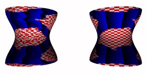 |
This image shows off both the reset_children warp and uv mapping. The lathe on the right has texture tex1 (see below), while the lathe on the left has texture tex2. Notice how the turbulence has been reset for the child textures, but still applies to the parent leopard pattern. Both are uv mapped. |
#declare Grad_tex = texture {
  pigment { gradient x color_map {[0 rgb <0,0,0>][1 rgb <0,0,1>]}}
}
#declare Check_tex = texture {
  pigment { checker rgb <1,1,1>, rgb <1,0,0> scale .25}
}
|
|
#declare tex1 = texture {
  leopard
  texture_map {
    [ .04  grad_tex]
    [ .06  check_tex]
  }
  warp { turbulence .3 }
  scale .1
}
|
#declare tex2 = texture {
  leopard
  texture_map {
    [ .04  grad_tex]
    [ .06  check_tex]
  }
  warp {turbulence .3 }
  warp {reset_children }
  scale .1
}
|
For those who care, the implementation of reset_children was two-fold. First, I added a new warp type called reset_children. Then, I added a parameter to Warp_EPoint so that it could know if it was warping the parent or the children patterns. If Warp_EPoint is warping a child texture and it hits a reset_children warp, it will stop. Since warps are applied in reverse order, this means that only the warps after the reset_children warp are used, which appears to the user as the child textures getting reset.
Author: Nathan Kopp
All textures in POV are defined in 3 dimensions. Even planar image mapping is done this way. However, it is sometimes more desirable to have the texture defined for the surface of the object. This is especially true for bicubic_patch objects and mesh objects, that can be stretched and compressed. When the the object is stretched or compressed, it would be nice for the texture to be "glued" to the object's surface and follow the object's deformations.
A new keyword has been added to object modifiers. If the modifier "uv_mapping" is specified, then that object's texture will be mapped to it using surface coordinates (u and v) instead of spatial coordinates (x, y, and z). This is done by taking a slice of the object's regular 3D texture from the XY plane and wrapping it around the surface of the object, following the object's surface coordinates.
Important: The "uv_mapping" keyword must be specified before the object is given its texture!
Important: With uv_mapped objects, it does not matter whether a texture is added to the object before or after the object's transformations!
a) The texture exists throughout <x,y,z> space. We take one slice from the plane z=0. For a lathe object, as shown here, we use the square where (u,v) = (0,0) through (1,1).
b) This shows a lathe object which is textured using normal mapping with a checker texture (the texture is scaled by 0.25 in every direction). It visualizes the texture being "wrapped" around the object.
c) Here we see the same lathe, but this time it is uv_mapped.
bicubic_patch
{
  <bicubic_patch specific stuff>
    .
    :
  uv_mapping

  texture { MyFavoriteWoodTexture }

  scale A
  rotate B
  translate C
}
Surface mapping is currently defined for the following objects:
Object |
Description |
| bicubic_patch | UV coordinates are based on the patch's parametric coordinates. They stretch with the control points. The default range is (0..1) and can be changed. |
| mesh, mesh2 | UV coordinates are defined for each vertex and interpolated between. |
| lathe, sor | modified spherical mapping... the u coordinate (0..1) wraps around the y axis, while the v coordinate is linked to the object's control points (also ranging 0..1). Surface of Revolution also has special disc mapping on the end caps if the object is not 'open.' |
| sphere | boring spherical mapping |
| box | image is wrapped around the box, as shown below. |
Some other objects that should eventually get surface mapping are: triangle, smooth triangle, cone, cylinder, superellipsoid, disc, height_field, plane, polygon, prism, and torus. If anyone wants to help me program with these, let me know.
Objects that will probably never get surface mapping are: blobs, julia fractals, cubic, polynomial, quadric, quartic, text, and isosurfaces (if these two patches are ever implemented concurrently).
Author: Nathan Kopp
Modified (4 corners for bicubic_patch) by: Mike Hough
I've added a new keyword, uv_vectors. This keyword can be used in bicubic patches (type 0, 1, 2 and 3) to set the UV coordinates for each of the four corners of the patch. This goes right after the control points and right before the texture. The default is
uv_vectors <0,0>,<1,0>,<1,1>,<0,1> // syntax is "uv_vectors <corner1>,<corner2>,<corner3>,<corner4>"
If you had another patch sitting right next to this (as happens often with sPatch or Moray), you could map the exact same texture to it but use something like
uv_vectors <1,0>,<2,0>,<2,1>,<1,1> // syntax is "uv_vectors <corner1>,<corner2>,<corner3>,<corner4>"
(depending on which side of this patch the other is on) so that the two textures fit seamlessly together.
This new keyword also shows up in triangle meshes (the original kind). Inside each mesh triangle, you can specify the UV coordinates for each of the three vertices uv_vectors <uv1>,<uv2>,<uv3>
This goes right after the coordinates (or coordinates & normals with smooth triangles) and right before the texture.
Example:
mesh {
  triangle {
    <0,0,0>, <0.5,0,0>, <0.5,0.5,0>
    uv_vectors <0,0>, <1,0>, <1,1>
  }
  triangle {
    <0,0,0>, <0.5,0.5,0>, <0,0.5,0>
    uv_vectors <0,0>, <1,1>, <0,1>
  }
  uv_mapping
  pigment {
    image_map {
      sys "AnImage"
      map_type 0
      interpolate 0
    }
  }
}
Note: The UV-mapping implemented here simply maps the X and Y of the texture to
the U and V of the object. It takes a slice of the texture from the XY plane (Z=0) and
wraps that slice around the object.
Any slice of gradient z parallel to the XY plane will have a uniform color, since the
texture will only change in the z direction.
The surface of an object is only 2 dimensional, whereas textures in POV are 3 dimensional.
At some point, only one slice of the 3d texture can be mapped to the 2d surface
coordinates.
You can use the XZ plane of a texture if you want to: you simply have to rotate the
texture so that the XZ plane lies in the XY plane.
rotate 90*x // this should do the trick
Author: Matthew Corey Brown
Syntax:
warp {
  cylindrical
  [ orientation VECTOR | dist_exp FLOAT ]
}
warp {
  spherical
  [ orientation VECTOR | dist_exp FLOAT ]
}
warp {
  toroidal
  [ orientation VECTOR | dist_exp FLOAT | major_radius FLOAT ]
}
defaults:
orientation <0,0,1>
dist_exp 0
major_radius 1
These warps essentially use the same mapping as the image maps use. This way we can wrap checkers, bricks hexagon and other patterns around spheres, toruses, cylinders and other objects. It wraps around the Y axis.
However it does 3D mapping and some concession had to be made on depth.
This is controllable by dist_exp (distance exponent). In the default of 0 imagine a box <0,0> to <1,1> stretching to infinity along the orientation vector. The warp takes its points from that box. (except for cylindrical where the y value doesn't get warped if you use the default orientation)
For a sphere distance is distance from origin, cylinder is distance from y-axis, torus is distance from major radius. (or distance is minor radius if you prefer to look at it that way)
However the box really is <0,0> <dist^dist_exp,dist^dist_exp>
This is for if you have a non torus, cylinder or sphere, the texture doesn't look stretched unless you want to.
Examples:
torus {
  1, 0.5
  pigment {
    hexagon
    scale 0.1
    warp {
      toroidal
      orientation y
      dist_exp 1
      major_radius 1
    }
  }
}
sphere {
  0,1
  pigment {
    hexagon
    scale <0.5/pi,0.25/pi,1>*0.1
    warp {
      spherical
      orientation y
      dist_exp 1
    }
  }
}
cylinder {
  -y, y, 1
  pigment {
    hexagon
    scale <0.5/pi, 1, 1> *0.1
      warp {
      cylindrical
      orientation y
      dist_exp 1
    }
  }
}
Syntax:
warp { planar [ VECTOR , FLOAT ] }
default:
warp { planar <0, 0, 1>, 0 }
This warp was made to help make the spherical, cylindrical, and toroidal act more like the 2D image mapping. It maps each point to a plane defined by a normal (the VECTOR) and offset (the float) just like defining a plane object.
Author: Nathan Kopp
When using a CSG difference to "cut" away parts of an object, it is sometimes desirable to allow the object to retain its original texture. Generally, however, POV will display the texture of the surface of the object that was intersected, which, in the case of a CSG difference, is the object that was used to do the cutting. Also, if that object was not given a texture by the user, the default texture is assigned to it.
By using the cutaway_textures keyword in a CSG difference, you can tell POV that you do not want the default texture to be assigned to the children of the difference, but instead, the textures of the other objects in the difference should be used. POV will determine which texture(s) to use by doing insidedness tests on the objects in the difference. If the intersection point is inside an object, that object's texture will be used (and evaluated at the interior point). If multiple textures are possible, then POV will average the textures together.
Syntax:
difference {
  <object_1_with_textures>
  <object_2_with_no_texture>

  cutaway_textures
}
Author: Chris Huff
warp { displace { PATTERN, COLOR_MAP } }
Displaces the pattern by an amount determined by the PATTERN and COLOR_MAP at each point. The rgb values are used as xyz displacement amounts.
Author: Mark Wagner
Support for the frequency and phase transformations is now extended to image_maps.
Author: Chris Huff
New pattern waveform:
atan_wave, compresses pattern values into the 0-1 range, no matter how
high they went previously.
Author: Ron Parker
The new keywords are:
MIN_EXTENT:
min_extent ( OBJECT_IDENTIFIER )
Returns the minimum x, y, z values for a #declared object. This is one corner of the object's bounding box.
Example:
#declare MySphere = sphere { <0, 0, 0>, 1 }
#declare BBoxMin = min_extent ( MySphere );
object {
  MySphere
  texture { pigment { rgb 1} }
}
sphere {
  BBoxMin, .1
  texture { pigment {color red 1} }
}
MAX_EXTENT:
max_extent ( OBJECT_IDENTIFIER )
Returns the maximum x,y,z values for a #declared object. One corner of the object's bounding box.
Example:
#declare MySphere = sphere { <0, 0, 0>, 1 }
#declare BBoxMax = max_extent ( MySphere );
object {
  MySphere
  texture { pigment { rgb 1} }
}
sphere {
  BBoxMax, .1
  texture { pigment {color blue 1} }
}
Both keywords are used in the same manner. The difference is that max_extent returns the largest components of the bounding box, while min_extent returns the smallest components.
To use these new functions, you must first #declare the object for which you wish to get extent information, as in this example:
// create a centered TrueType text shape
#declare Newtext =
text {
  ttf "crystal.ttf", "Bound", 1, 0
  scale 3*y
  pigment {Red}
}
#declare transvect = -x * max_extent (Newtext).x/2
object {Newtext translate transvect}
This code creates a TrueType text object, then centers it on the origin along its X axis.
Be sure to view the normal bugfix and layered textures sections for more information about those two significant changes.
Author: Nathan Kopp
The most prominent manifestation of this bug is incorrect surface normals when normals are combined using an 'average' pattern. This has been fixed.
Author: Nathan Kopp
When reflection is used on a surface with a perturbed surface normal, the reflected rays sometimes go through the object instead of bouncing off of it. This has been fixed. This bugfix is now part of the official version.
Author: Nathan Kopp
2-d vectors are treated as floats and not vectors. To fix this, all 2-d vectors are automatically promoted to 3-d vectors.
Author: Gerald K. Dobiasovsky
This patch fixes some bugs in the ultra_wide_angle and cylinder cameras.
Author: Nathan kopp
Fixed cylinder cameras again. (v. 0.6)
In POV 3.1, some objects were double-illuminated (the backside of a surface was illuminated by light hitting the opposite side) by default. This 'feature' was actually a work-around for another bug that was fixed. Therefore, double-illumination is now not enabled by default on any object. See the double_illuminate section for more information on how to re-enable double-illumination. As of MegaPov 0.5, double illumination is also disabled for smoothed heightfields by default.
Authors: Burton Radons, Nathan Kopp, Smellenbergh
Macro performance has been greatly enhanced in MegaPov. Macros are loaded into memory, meaning that the file system is used much less. Macros are only loaded if necessary, which even further improves performance.
Authors: Smellenbergh, Nathan Kopp
Memory allocation caches have been implemented to avoid calling "malloc" and "free" during the main ray-tracing loop. This can greatly improve performance, depending on the speed of the operating system's memory allocation routines.
Author: Nathan Kopp (with assistance of Alexander Enzmann)
The fractal noise function in POV-Ray contained bugs which caused 'plateaus'. By suggestion of Alexander Enzmann, the function has been modified to reduce its range so that clipping does not produce plateaus anymore. This will affect the pigments: crackle, wrinkles, bozo, and bumps. It should not affect the wrinkles, bumps, or dents when used as normals.) It also affects the isosurface noise3d function, as well as turbulence.
Note: Set the version to #version unofficial MegaPov 0.5; to use this fix. Lower version numbers will make MegaPov use the old style.
Author: Various
Due to potential legal issues regarding a U.S. patent held by Unisys covering LZW compression and decompression, GIF support has been removed from MegaPov. This was done to legally protect the authors and distributors of MegaPov from potential lawsuits. Your thoughtful understanding of the necessity of this action is greatly appreciated.
You can use gif2png (which can currently be downloaded from http://www.tuxedo.org/~esr/gif2png/ or http://pegasus.uni-paderborn.de/enno/burnallgifs/ to convert your GIF images to PNG images.
Please read the Unisys statement about the LZW patent.
Here is a quote from that statement (emphasis added, quoted in June, 2000):
Here is another quote from that statement (emphasis added, quoted in June, 2000):
As a hobbyist, I (Nathan) do not have the time (or money) to hire a lawyer to speak to a Unisys representative in a (most likely futile) attempt to obtain a free license to legally use GIF decompression technology.
Author: Mark Wagner
When using image_maps with transmit all or filter all, 24 bit PNG images caused a crash.
Not only has this been fixed but 24 bit images can be used now.
pigment {
   image_map {
      png "a 24bit_png.PNG"
      map_type 0
      interpolate 0
      filter all 0.6
   }
}
Note: this doesn't change anything for indexed images. These can only be used with images supporting palettes.
Author: Nathan Kopp
When transforming the mesh in space (rotation/translation...), the textures were not transformed as well. This only affected the corner-interpolated meshes. It has been fixed now.
Author: Smellenbergh
New keywords for animation. These new keywords allow you to use the values of the clock rendering options in your scene source: If used correctly, you will only need to change the clock settings and your scene source will use the new clock settings.
Note: These values are the ones after being adjusted by POV-Ray. So, if the option 'cyclic animation' is set, they could be different from the ones given in the dialog.
Author: Ronald L. Parker
In the official POV-Ray, it is possible to determine whether a variable has been declared but it is not possible to check whether a specific element of an array has been declared. Now a patch allows such a check.
Example:
#declare Myarray = array [10]
...
#ifdef (Myarray [0] )
...
#end
Author: Chris Huff
eval_pigment
(PIGMENT, VECTOR)This function returns the color (rgb) of a pigment at an evaluation point.
PIGMENT: use the identifier for the declared pigment or the full pigment to be evaluated.
VECTOR: the point in 3d-space to be evaluated. Combine it with the trace function to find points on the surface of the object.
eval_pattern
(pattern, vector) functionThis function returns the float value of the pattern at the evaluation point.
Author: David Sharp
Hyperbolic trig functions
These take a float as parameter and return a float:
cosh(a), sinh(a), tanh(a), acosh(a), asinh(a), atanh(a);
Complex functions
Complex numbers in these functions are just 2-d POV scene language vectors where the real part is the x (or u) coordinate and the imaginary part is the y (or v) coordinate. For example,
#declare cmplx1=<1,.5>;
#declare cmplx2=<.2,-2>;
represent the complex numbers 1 + .5*i and .2 + -2i
These take 2-d POV scene language vector(s) <real,imag> as parameters and return a 2-d scene language vector <real,imag>.
They are the complex versions of the real number functions without the initial 'c' in the function name.
These functions take 2-d POV scene language vector(s) <real,imag> as parameters and return a float.
Author: from TMPov
The "hf_height_at" function returns the height of a height_field at a given position on the height_field.
It has the following syntax:
hf_height_at (XCOORD, ZCOORD, IDENTIFIER)
XCOORD and ZCOORD are both in the range of 0 to 1 and represent the position you want to test on the height_field.
IDENTIFIER is the declared height_field object to test.
hf_height_at returns a number in the range of 0 to 1.
EXAMPLES:
#declare Myhf = height_field { tga "field.tga" translate <-0.5,0,-0.5> scale <20,5,20> }
#declare Ypos = hf_height_at ( 0.5, 0.5, Myhf )
The above example would return the height at the center of the height field object. This number would be from 0 to 1, so, in the above example, Ypos would need to be multiplied by 5 to get the actual height of the point (since Myhf was scaled by 5 in the y-direction). This function can be used to put trees and other objects on terrain, for instance.
Author: Smellenbergh
Two new keywords have been added so that the image size given in the rendering options can be used in your scene source
image_width //reads the +Wn value
image_height //reads the +Hn value
When using those keywords to set the camera ratio (up and right vectors) the viewing angle of the camera will always cover the full width of the rendered image. No matter which image sizes are used, the image will always show the right proportions. Use it like this:
up y*image_height
right x*image_width
A way to ensure that an intended image ratio of 1/1 is used when rendering could be done this way:
force the image heigth to be the same as the image width through the ini_option in the global_settings.
global_settings {
  ini_option concat("Height=",str(image_width,0,0))
}
You could also make some items of the scene dependent on the image size:
#if (image_width < 300) crand 0.1 #else crand 0.5 #end
or:
image_map {
  pattern image_width, image_width { //make resolution dependent of render width
    gradient x
    color_map { [ 0.0 ... ] [ 1.0 ... ] }
  }
}
Author: Nathan Kopp
Note: The ini_option will probably be discontinued in the future.
You can specify some options that usually go in INI files in a POV file by using the 'ini_option' keyword. The ini_option keyword followed by a string containing the option should be placed in the global_settings {} block in your POV file.
Here are some examples:
global_settings {
  ini_option "Height=640"
  ini_option "Width=480"
  ini_option "+QR" // turn on radiosity
}
Not all INI options can be used. Specifically, those related to animation, output file, and shell-out commands are not allowed.
Author: Nathan Kopp
One of my pet peeves with POV is the inability to redefine an identifier as another type of identifier. This causes problems with #local variables, too, since they must be of the same type of any perviously-declared variables of the same name. UVPov currently has been changed to allow users to redefine identifiers any time. #local variables can be of another type but still do not destroy the variable with the larger scope.
Author: Nathan Kopp
Instead of using #declare, use $. Instead of using #local, use %.
So if your code used to look like:
#declare a = 100;
#declare b = a*sqrt (2);
#local c = object {my_object rotate 20}
it could now look like:
$a = 100;
$b = a*sqrt (2);
%c = object{my_object rotate 20}
You can still use #declare and #local if you so choose.
STRING_ENCODING:
place this in the global_settings { }:
string_encoding "UTF8" | "ISO8859_1" | "Cp1252" | "MacRoman"
specifies the encoding used for extended character sets. This is currently only used for text objects, but may be extended to other string manipulation functions in the future. The double quotes are required. The default encoding is UTF8.
Author: Yvo Smellenbergh
With the new keyword date, time and/or a date can be used in your images.
This might be useful in a macro to place a time stamp in your images, along with your name.
The new keyword date works like other string functions, except that you have to supply a format string.
Example (Suppose it's saturday 1 january):
#declare TheString=date("%a %B")
Will return the string: Sat January
We have chosen for the most flexible way (which is probably not the easiest ...) because not all countries write dates in the same way. Just think of the difference between the USA and most parts of Europe.
These are the possible specifiers for the format string:
Please note that these should be equal for all platforms but if you don't get the expected result, contact the person who compiled your version to find out if there are differences.
These following descriptions are for MacMegaPov.
Char Description
Note: To use the '%' character in the result, use it twice: date("%%")
Refer to date.pov for an example scene.
Please note that you might have to write the result in a file if you want to abort the rendering and continue later on. Otherwise you could get a different result because time goes on :-)
The keyword start_chrono sets an internal variable and returns the current internal clock counter.
The return value is not important. However, you must assign the return value from start_chrono otherwise you get an error.
Use it like this:
#declare Dummy=start_chrono; //this is ok
or use it like this:
#if ( start_chrono) //this is also ok
but not:
start_chrono //parsing stops with a fatal error
The keyword current_chrono returns the time in seconds between start_chrono and current_chrono. The start value is not changed, a second current_chrono will still return the seconds between start_chrono and the second current_chrono.
If you don't call start_chrono somewhere before you call current_chrono, you will get the seconds elapsed since the beginning of the current render.
Example:
#declare ParseStart= start_chrono; //resets the chrono and returns the internal clock counter
... syntax to be parsed
#declare ParseEnd= current_chrono; //reads the seconds elapsed since chrono_start
#debug concat ( "\nParsing took ", str((ParseEnd , 5, 5), " seconds\n")
Refer to chrono.pov for a demo scene.
tick_count
returns the the current internal clock counter, it has no effect on the chrono. Unlike start_chrono, the counter is not reset.tick_count increases by 60 times per seconds on a Macintosh, but other platforms have other values.
A value of 200 is common for Atari and if I'm not mistaken, 1000 for Intell-based machines.
This keyword could be used to call a seed number that will be different for each render, thus making the rand() function random for each render.
See truerand.pov for an example of tick_count.
Author: Ronald L. Parker
SYNTAX:
trace ( OBJECT_IDENTIFIER, <Start>, <Direction>, [VECTOR_IDENTIFIER] )
Traces a ray beginning at <Start> in the direction specified by <Direction>. If the ray hits the specified object, this function returns the coordinate where the ray intersected the object. If not, it returns <0,0,0>. If a fourth parameter in the form of a vector identifier is provided, the normal of the object at the intersection point (not including any normal perturbations due to textures) is stored into that vector. If no intersection was found, the normal vector is reset to <0,0,0>.
Note: Checking the normal vector for <0, 0, 0> is the only reliable way to determine whether an intersection has actually occurred, intersections can and do occur anywhere, including at <0,0,0>.
Example:
#declare MySphere = sphere { <0, 0, 0>, 1 }
#declare Norm = <0, 0, 0>;
#declare Start = <1, 1, 1>;
#declare Inter=
trace ( MySphere, Start, <0, 0, 0>-Start, Norm );
object {
  MySphere
  texture {
    pigment { rgb 1}
  }
}
#if (Norm.x != 0 || Norm.y != 0 || Norm.z != 0)
cylinder {
  Inter, Inter+Norm, .1
  texture {
    pigment {color red 1}
  }
}
#end
Author: Chris Huff
The transform patch does two things: First, it allows you to invert any transform
by adding "inverse" to the transform {...} block. An inverse transform
does the opposite of what it would normally do, and can be used to "undo"
transforms without messing around with huge numbers of transformations. To do the same
without this patch, you would have to duplicate each transform, change them to do the
opposite of what they would normally do (like "translate -y*3" instead of
"translate y*3"), and reverse their order.
Second, it allows transform {...} blocks to be placed anywhere an ordinary transform can
go. The previous syntax was:
object/pigment/etc {
  transform TRANSFORM_IDENTIFIER
}
This is still supported, but the new syntax is:
object/pigment/etc {
  transform {
    TRANSFORM_IDENTIFIER
    TRANSFORMATIONS(translate, rotate, scale, matrix, transform)
  }
}
And you can have multiple transform {...} blocks, they are done in order, as expected. This also means you don't need to use vinv_transform, you could use vtransform(VECTOR, TRANSFORM inverse) instead. The vinv_transform() patch predated the transform patch.
Originally, turbulence was created to modify textures, but I've made it available for you. The formula is:
vturbulence ( Lambda, Omega, Octaves, InVec)
It returns a vector which you can scale and add to InVec and have a turbulated vector. A rope made of blobs and being straight can be perturbed by turbulence.
The meaning of the Lambda, Omega and Octaves parameters could be found in the original Pov docs.
The biggest advantage of turbulence is that the points near each other have similar turbulation.
Author: Chris Huff
The syntax is:
vtransform (VECTOR, TRANSFORM)
Where VECTOR is the point to be transformed and TRANSFORM is any standard POV-Ray transform (scale, rotate, translate, matrix, transform {}...).
vinv_transform (VECTOR, TRANSFORM)
Where VECTOR is the point to be transformed and TRANSFORM is any standard POV-Ray transform (scale, rotate, translate, matrix, transform {}...). The vinv_transform function returns the result of applying the inverse(reverse) of TRANSFORM to VECTOR. In other words, it undoes the effect of applying a transform.
Author: Chris Huff
vwarp(POINT, WARP)
Applies a warp to a given vector. See the POV-Manual for an explanation of how warps work, and you will understand what this function does.
Author: Chris Huff
noise3d( VECTOR_POINT )
This is identical to the noise3d() function in isosurfaces, but it is now available in ordinary scene code.
Author: Phil Carrig
This patch renders a POV-Ray animation directly into a density (.df3) file.
You can create a density file of an object by having each frame render a slice of the object.
Set your scene up for rendering an animation. Use +fd or Output_File_Type=d as the output file type (in the original POV-Ray this meant 'dump' format but this is no longer supported).
If an output file does not exist or if an existing file has different dimensions than requested for this render a new file will be created. This will be a full size df3 file which will be all zeros. Otherwise the render output will be inserted into the existing file. The reason I did this is that you can render some of the slices in one render session and then complete it in another render session.
Lets say you want a 100x100x100 df3 file. You'd set the image size to 100x100 and the animation frame range to 100 frames. If you set the subframe range to 20..80 for example you'd still get the full 100x100x100 df3 file but the slices 0..19 and 81..99 would be whatever was already in the file or zeros if it's a new file.
Another example. You have used the above settings 100x100 image size and 100 frames and you abort the render after 50 frames. You can complete the df3 file by setting the Subset_Start_Frame to 50 and restarting the render.
The output values are a greyscale representation of the pixel colors using the formula Red*0.3+Green*0.11+Blue*0.59
Some other points.
If the output is sent to standard output then it will be sent as a stream. i.e. the renderer won't try to create a complete empty file.
I have no idea what happens if you try to use antialiasing.
Authors: Marcos Fajardo, Chris Huff
New atmospheric glow effects:
This makes a fast-rendering glow effect. It is based on the light source glow effect from POV-AFX,
written by Marcos Fajardo, but has been heavily modified.
Syntax
glow {
  type 0 | 1 | 2 | 3
  location LOCATION
  size FLOAT_SIZE
  radius FLOAT_RADIUS
  fade_power FLOAT_POWER
  color COLOR
  WARPS
  TRANSFORMS
}
You can specify glows individually, or attached to a light_source. If created in a light source, they will be automatically initialized with the light's position and color (though transforming the light source will not give the expected result).
Choose a glow "type" from 0, 1, 2 or 3. Type 2 and 3 glows are not completely implemented yet, but 2 will be based on the exp() function and 3 will simulate a sphere with constant density.
The "size" keyword adjusts the scale of the glow effect. It is not an absolute size, just a scaling amount (because some glows are infinite). It does not quite work properly yet, it causes strange effects with changing distances of objects behind the glow.
The "radius" keyword specifies a clipping radius confining the glow to a circular area perpendicular to the ray. If the glow is still visible at this radius, it will make a sudden transition.
The "fade_power" keyword allows you to provide an exponent to adjust the falloff with.
Author: Nathan Kopp
One part of POV that gets a lot of complaints is its radiosity. But when it is used correctly, you can usually produce some very nice images. Unfortunately, there are a few bugs and limitations to the implementation of radiosity in the official release of POV-Ray 3.1.
First, I guess I should say that, as the POV-Ray manual points out, POV-Ray does not use "real" radiosity. True radiosity renderers convert the entire scene to polygons, and then compute a lighting solution by approximating a solution to a huge set of linear equations.
POV's solution to radiosity is sometimes known as monte-carlo ray-tracing. When an eye ray hits an object and POV wants to know how much indirect light is hitting the surface, it shoots out a bunch of random rays into the scene and "gathers" light from the other objects.
Obviously, it would be very bad to do this for every intersection. One assumption that can generally be made about indirect diffuse light is that it doesn't change very quickly. So a good approximation is to shoot lots of rays from a small percentage (usually between 1 and 5%) of the intersections and then interpolate between those values.
In Warp's radiosity tutorial (http://www.students.tut.fi/~warp/pics/Radiosity_test2/comments.html), his first rule is, "Choose your ambient light carefully." Warp's explanation demonstrates how, in the official POV 3.1, the brightness of radiosity is greatly affected by ambient_light settings.
So what does orthogonal mean? That just means that the two features are independent and affect each-other in well-defined and expected ways. This is not the case of the official release of POV-Ray 3.1.
The brightness of radiosity in MegaPov is based on two things:
1) the amount of light "gathered"; and
2) the 'diffuse' property of the surface finish.
An object can have both radiosity and an ambient term. However, I suggest that if you use radiosity in a scene, you either set ambient_light to 0 in global_settings, or use ambient 0 in each object's finish. This lighting model is much more realistic, and POV will not try to adjust the overall brightness of the radiosity to match the ambient level specified by the user.
To use exaggerated radiosity, increase the 'brightness' in the radiosity section of global_settings, instead of turning up ambient_light.
First, in order to get good interpolation, you should get a bunch of points and interpolate those. POV-Ray allows you to specify a "nearest_count" which, according to the documentation, is the "maximum number of old ambient values blended together". Unfortunately, this means that sometimes you might end up blending only one value. Averaging one value with itself can lead to a bad approximation.
Therefore, in MegaPov, use nearest_count to specify the minimum number of old values blended together. The total number blended will vary depending on error_bound. All previous values that fit within the specified error_bound will be used in the average.
I always thought the explanation of distance_maximum in the documentation was difficult to understand.
When looking in the code, I noticed that if you don't specify a distance_maximum, POV will estimate based on the distance from the camera to the first intersection. I extended this concept and compute distance_maximum for every intersection automatically based on the distance from the camera. It's worked wonderfully in all of my tests. If you specify a distance_maximum, it will be ignored.
Warp's second rule in his radiosity tutorial is, "Don't make your room too big." The reason that any sized rooms will work is because of this auto-computation of distance_maximum as well as a big bug fix relating to error_bound and the first radiosity pass. Together, these work to remove much of the splotchiness that plagued radiosity in the past.
You can specify any recursion_limit that you wish (after about 5 or 6, it gets pointless, though... well, except for maze-like scenes).
If you have a clear object, you'll get radiosity on the other side. If you have a mirror, the reflected image will show radiosity.
You can specify an adc_bailout for radiosity rays. Use adc_bailout = 0.01 / brightest_ambient_object for good results.
Fixed a bug relating to error_bound and samples stored during the first radiosity pass.
Radiosity estimation can be affected by surface normal. To enable this feature, add normal on to the radiosity {} block within global_settings {}.
Radiosity estimation can be affected by media. To enable this feature, add media on to the radiosity {} block within global_settings {}.
You can save the radiosity data using save_file "file_name" and load the same data later using load_file "file_name". Be aware that this is not fully tested, and thus artifacts may appear. Also, as with saving and loading of photon data, it is not a good idea to save and load radiosity data if scene objects are moving.
Even if data is loaded, more samples may be taken during rendering (which produces a better approximation). You can disable samples from being taken during the final rendering phase by specifying always_sample off. Note that this feature can be used even if data is not loaded, and may reduce splotchiness.
Instead of using the INI options "Preview_Start_Size" and "Preview_End_Size" to control the radiosity pre-trace gathering step, use the keywords pretrace_start and pretrace_end within the radiosity block inside global_settings. Each of these is followed by a decimal value between 0.0 and 1.0 which specifies the
In the official version of POV 3.5, specifying "+QR" on the command line would enable radiosity even if radiosity {} was not specified in the POV file's global_settings. Thus, the radiosity quality setting could not be enabled by default, since it would enable radiosity for all scenes. In MegaPov, you can specify "+QR" in your default INI file, and the feature will only be enabled if radiosity {} is specified in the POV file's global settings.
Sometimes there can be problems with splotchiness that is caused by objects that are very bright. This can be sometimes avoided by using the max_sample keyword. max_sample (which is placed within the radiosity block inside global_settings) takes a float parameter which specifies the brightest that any gathered sample is allowed to be. Any samples brighter than this will have their brightness decreased (without affecting color). Specifying a non-positive value for max_sample will allow any brightness of samples (which is the default).
Medium-quality radiosity can be enabled simply by adding:
global_settings { radiosity {} }
Simply specifying radiosity {} will enable the feature. The default settings are generally good, and are the same as the "medium quality" settings shown below.
This code works for most scenes:
#declare high_quality=no; // or yes
#if(high_quality)
  // High Quality - slow rendering
  ini_option "+QR"

  radiosity{
    pretrace_start 0.08
    pretrace_end   0.02
    count 80             // CHANGE range from 20 to 150
    nearest_count 5      // CHANGE range from 3 to 10
    error_bound 1        // CHANGE - range from 1 to 3 - should correspond with pretrace_end
                         //   1 : pretrace_end = 0.02
                         //   3 : pretrace_end = 0.08
                         //   use pretrace_start = 0.08
                         // you can go lower than 1, but then you probably will want to set
                         // pretrace_end to 0.01, which is really slow
    recursion_limit 4    // CHANGE

    low_error_factor .5  // leave this
    gray_threshold 0.0   // leave this
    minimum_reuse 0.015  // leave this
    brightness 1         // leave this

    adc_bailout 0.01/2   // CHANGE - use adc_bailout = 0.01 / brightest_ambient_object
  }
#else
  // Medium Quality - works for most scenes
  ini_option "+QR"

  radiosity{
    pretrace_start 0.08
    pretrace_end   0.04
    count 35             // CHANGE range from 20 to 150
    nearest_count 5      // CHANGE range from 3 to 10
    error_bound 1.8      // CHANGE - range from 1 to 3
    recursion_limit 3    // CHANGE

    low_error_factor .5  // leave this
    gray_threshold 0.0   // leave this
    minimum_reuse 0.015  // leave this
    brightness 1         // leave this

    adc_bailout 0.01/2   // CHANGE - use adc_bailout = 0.01 / brightest_ambient_object
  }
#end
Sometimes extra samples are taken during the final rendering pass.
These newer samples can cause discontinuities in the radiosity in some scenes. To decrease these artifacts, use a pretrace_end of 0.04 (or even 0.02 if you're really patient and picky). This will cause the majority of the samples to be taken during the preview passes, and decrease the artifacts created during the final rendering pass. You can force POV-Ray to only use the data from the pretrace step and not gather any new samples during the final radiosity pass. To do this, use "always_sample no" within the radiosity block inside global_settings.
If your scene uses ambient objects (especially small ambient objects) as light sources, you should
probably use a higher count (around 100 is usually good, but for final renders probably 150). For such scenes, an error_bound of 1.0 is usually good. Higher causes too much error, but lower causes very slow rendering
The medium quality setting above is usually good for scenes with an average amount of diffuse illumination. It renders fairly quickly and gives good results.
If things look splotchy in your scenes, increase the count and nearest_count.
Author: Nathan Kopp
You can turn on persistent variables by adding the following line to the INI file used to generate your scene:
Persistent_Animation=yes
With this option, all variables will be persistent throughout the animation. This means that they are not destroyed at the end of one frame. They remain in existence until the render is finished or interrupted. Continuing a render (with the continue trace INI option) will not restore variables. Remember, you can undefine variables with #undef if you want to delete them. You can also redefine a variable to a different type with UVPov.
Note: There is currently no command-line option that corresponds to this INI option.
The Persistent_Animation option also enables persistent scene objects.
Usually, when a frame is finished being rendered, POV will destroy all objects in the scene. UVPov gives you the ability to add labels to objects in your scene. When Persistent_Animation is enabled, all frame-level objects that have labels will remain at the end of the frame and will not be destroyed
You can label an object with the 'label' keyword as an object modifier. Use it just as you would use 'translate' or 'rotate'. For example:
union{
  sphere{ 0,1 texture{myTex}  label mySphere }
  box{-1,1 texture{myTex2} label myBox }
  label myCsg
}
Notice that no quotes are placed around the label. Any word can be used as a label (even reserved keywords such as sphere or x). Objects can share labels.
It is important to realize that object labels are in a completely different namespace than #declare or #local names. You cannot use object labels where POV is expecting a #declared object, nor can you use a #declared object name where POV is expecting an object label. Also, object labels only become effective when the object is part of the scene. If it has simply been #declared and given a label, you cannot use the modify{} or delete{} modifiers described below until it is placed in the scene.
Once you have labeled an object, it will be persistent throughout the animation. When a frame has been rendered, the object will not be deleted before the next frame is parsed.
You may want to modify a persistent object. You can do so with the 'modify' keyword. Here's an example:
modify{
  myCsg
  translate 10*x
}
If multiple objects share this label, the object modifiers will be applied to all of them.
Note: the POV code for the object modifiers is re-parsed for each object that they are applied to. For this reason, if you use random numbers in the modify{} block, each object that is modified will be modified differently. Think of it like a #while loop that is automatically created that repeats for all objects that have that name.
You can delete a labeled object also:
delete { myCsg }
Finally, you can modify or delete a labeled object object within a labeled CSG object. To do so, use a period to separate the names (like object-oriented programming). Here's how:
modify{
  myCsg.myBox
  texture{myTex3}  // apply a new texture
}
In the future, I want to add modifiers that allow you to add new children to a CSG object and replace one object with another.
Author: Nathan Kopp
Starting with MegaPov 0.4, post processing is available. In version 0.4, three post-processing 'effects' were created: depth, focal_blur, and soft_glow. The syntax of these three effects is likely to change, but the concept will remain the same. In MegaPov 0.5, a host of other filters have been introduced. The math operators have been expanded in MegaPov 0.6.
Post-processing modified the rendered image after the ray-tracing step has completed. In the past, post-processing of POV images required third-party software (such as PhotoShop, Paint Shop Pro, or the GIMP). With post-processing capabilities built in to POV, the type of effects available is greatly expanded (for example, focal_blur effect, which uses depth information).
Multiple effects can be applied to a scene, and they are applied in the order that they are specified.
global_settings {
  :
  [POST_PROCESS_BLOCK]
  :
}

POST_PROCESS_BLOCK:
  post_process {
    [overwrite_file]
    [keep_data_file]
    [POST_PROCESS_EFFECTS...]
  }

POST_PROCESS_EFFECT:
  clip_colors { COLOR_MIN, COLOR_MAX } |
    :  |
  stars {DENSITY, COLOR_RANGE_MIN, COLOR_RANGE_MAX}
overwrite_file: If you specify overwrite_file, POV will replace the original file with the post-processed version. Otherwise, POV will write the post-processed file to a new file with the same name, but with "_PP" appended to the end of the file name.
keep_data_file: If you specify keep_data_file, the temporary file with the additional data (depth, normal, ...)
will not be trashed after the postprocessing, but saved in the same folder as the image file. It will get the same name as the image, but with
the extension .ppd (Post Process Data). Note: Do not use overwrite_file with this option, since it will overwrite your unprocessed image.
This option is useful if you want to try out different post_process effects on an image that took forever to render. Set to
continue and render again with a different post_processing effect.
Multiple Effects: Multiple effects can be applied to the same file. Here is an example where both depth and focal_blur are applied to the same image.
global_settings {
  post_process {
    depth {0, 100}
    focal_blur{ 25, 30, 6}
  }
}
Author: Chris Huff
Syntax:
clip_colors { COLOR_MIN, COLOR_MAX }
Example:
clip_colors { color rgb < 0.5, 0, 0.5>, color rgb < 1, 0.2, 1>}
Clips all colors in the image between color_min and color_max.
Author: Chris Huff
Syntax:
color_matrix { <AA, AB, AC, BA, BB, BC, CA, CB, CC> }
Example:
color_matrix {
     < 0.5, 0.75, 0.25,
       0.5, 0.75, 0.25,
       0.5, 0.75, 0.25 > }  //black-white
Runs the color through a 3*3 matrix. The equation is:
R = r*AA + g*AB + b*AC
G = r*BA + g*BB + b*BC
B = r*CA + g*CB + b*CC
Where the matrix is:
 < AA, AB, AC,
   BA, BB, BC,
   CA, CB, CC >
Author: Chris Huff
Syntax: convolution_matrix { XDIM, YDIM, DIVISOR, LEVELING, <MATRIX_VALUES...> }
Example:
convolution_matrix {9, 1, 9, 0,
  < 1, 1, 1,
    1, 1, 1,
    1, 1, 1 >
}
Multiplies the pixel and the adjacent pixels (in the area defined by the matrix size) by the respective values in the matrix, adds the results together, and divides by DIVISOR to get an average color. A leveling value can be added in before the final division.
Another Example:
convolution_matrix {9, 1, 9, 0,
  < 1,  1, 1,
    1, -8, 1,
    1,  1, 1 >
}
This matrix finds the edges based on color in an image.
The depth effect converts the image to a grey-scale depth rendering.
example:
global_settings {
  post_process { depth {0, 100} }
}
This will produce a grey-scale image with pure white at a depth of zero and black for depths of 100 and greater.
Authors: Chris Huff and Nathan Kopp
Syntax:
find_edges {
  DEPTH_THRESH, NORMAL_THRESH, COLOR_THRESH,
  LINE_RADIUS, SHARPNESS, PIGMENT_STATEMENTS
}
Finds the edges in an image using depth, normal, and color information. Separate thresholds are specified for each of the three methods of edge detection:
The width of the lines is controlled by the line_radius parameter. The sharpness of the lines is controlled by the sharpness parameter. A sharpness of 1.0 yields nicely anti-aliased lines. A sharpness value of 0.0 leads to blurry lines when larger radii are used, and a sharpness value of greater than 1.0 begins to remove anti-aliasing from the lines.
The color of the line is controlled by the pigment specified. This pigment is evaluated over the range of <x,y> = <0,0> ... <1,1> (with z=0) over the full size of the image. Using solid colors is usually a good idea, unless special effects are desired.
Example:
find_edges {
  1, .3, .15, 2, 1.0, rgb 0
}
Finds edges wherever there is a depth difference greater than 1.0, a normal difference greater than 0.3 (about 60 degrees), or a color difference of 0.15. It uses a line radius of 2.0, with black (rgb 0) antialiased (sharpness 1.0) lines.
Author: Nathan Kopp
The focal blur effect adds a depth-based focal blur effect to the image.
example:
global_settings {
  post_process { focal_blur { 25, 30, 6} }
}
Here, the center of the focal range center is at a distance of 25 units, and it is 30 units wide. Therefore, all objects between 10 and 40 units are completely in focus. The maximum blur amount for the gaussian blur is a radius of 6 pixels.
Author: Chris Huff
Syntax:
invert
Inverts the colors of the image, using the equation: color = 1-color (computed separately for each r,g,b channel)
These should be pretty self-explanatory, they perform the operation they represent on each pixel, channel by channel. They can be controlled by a pigment for even more control.
The pigment is applied to the image as though the upper left corner is < 0, 1, 0> and the lower right is < 1, 0, 0>. This means image_maps are automatically centered on the image.
Author: Chris Huff
Syntax:
add { PIGMENT_STATEMENTS}
Examples:
add { bozo color_map {[0 Green][0 White]}}
Author: Chris Huff
Syntax:
divide { PIGMENT_STATEMENTS}
Divides the colors of the image by the colors of the pigment.
Examples:
divide { gradient y color_map {[0 Green][0 White]}}
Author: Chris Huff
Syntax:
exponent { PIGMENT_STATEMENTS }
Examples:
exponent { rgb 1 }
Author: Chris Huff
Syntax:
multiply {PIGMENT_STATEMENTS}
Examples:
multiply { color rgb < 0.5, 0.5, 1>}
Author: Chris Huff
Syntax:
post_min {PIGMENT}
Author: Chris Huff
Syntax:
post_max {PIGMENT}
Author: Chris Huff
Syntax:
subtract {PIGMENT_STATEMENTS}
Subtracts a pigment from the image.
Examples:
subtract { color rgb < 0.5, 0.5, 1>}
Author: Chris Huff
Syntax: normal
Example: normal
Displays the unperturbed normal values as rgb colors. The normals are scaled to the 0-1 range, so <-1,0,0> is rgb <0,0.5,0.5>.
Author: Chris Huff
Syntax:
patterned_blur { BLUR_DISTANCE, BLUR_DIVISOR, LEVELING, PIGMENT_STATEMENTS }
Example:
patterned_blur {12, 0, 0,
    bozo
    color_map {[0 rgb 1][0.15 rgb 0][1 rgb 0]}
    scale 0.05
}
Blurs the image by an amount depending on a pigment. Note that (unlike blur_matrix), it is automatically divided by the number of samples, so use a divisor and leveling value of 0 to have plain blur.
Author: Chris Huff
Syntax: posterize { COLOR }
Example:
posterize { color rgb 5 }
Divides the colors of the image into separate steps. The color parameter specifies the number of steps per channel.
The soft glow effect produces a nice soft-glow on the image by applying a gaussian blur to the image, and then combining that with the original image using a 'lighten' combination.
Example:
global_settings {
  post_process { soft_glow {1.0, 8} }
}
This is a standard soft glow effect, with a strength of 1.0 and a gaussian-blur radius of 8.
Author: Chris Huff
Syntax:
stars {DENSITY, COLOR_RANGE_MIN, COLOR_RANGE_MAX}
Example:
stars {0.05, rgb < 0.6, 0.8, 0.7>, White}
Replaces any background or sky_sphere areas with a non anti-aliased starfield.
Author: Nathan Kopp
First, you can disable all of these changes and revert to the way the original version handles normals by using "#version official 3.1;" at the end of your POV file.
This change affects the way normals are affected by transformations and warps. In general, it causes POV to act consistently when normals are scaled.
If you scale a normal, the apparent depth of the bumps will also scale, causing the slope to remain the same. You can disable this feature with the keyword "no_bump_scale". You can scale the normal non-uniformly to create a non-uniform scaling of the apparent depth of the bumps, as well.
They say a picture is worth a thousand words, so take a look at my page on Surface Normal Behavior: http://nathan.kopp.com/normals.htm (there are a number of pictures which explain what is going on).
When applying warps to a normal pattern, it is important to understand that the warp will only have an affect in determining which point in the pattern is used. For most cases, this will work as expected. However, in patterns that have flat places (areas with constant slope), such as crackle, adding warps such as turbulence will not change the slope. The turbulence will cause a different point to be used, but if that point has the same slope as the original point, the normal would be the same as if no turbulence was applied.
In general, if you want to add bumpiness, it is better to average a granite normal with your original normal instead of using a turbulence warp. Although in some cases in the official version, you can add bumpiness by using turbulence, it often produces the same results as MegaPov. Again, you can use #version official 3.1; if you need to revert to the behavior of the original version.
If you want to turn off bump scaling for a texture or normal, you can do this by adding the keyword "no_bump_scale" to the texture's or normal's modifiers. This modifier will get passed on to all textures or normals contained in that texture or normal. Think of this like the way no_shadow gets passed on to objects contained in a CSG.
It is also important to note that if you add "no_bump_scale" to a normal or texture that is contained within another pattern (such as within a texture_map or normal_map), then the only scaling that will be ignored is the scaling of that texture or normal. Scaling of the parent texture or normal or of the object will affect the depth of the bumps, unless "no_bump_scale" is specified at the top-level of the texture (or normal, if the normal is not wrapped in a texture).
Note: Using no_bump_scale will not give the same results as the official version. To get the exact same results as the official version, you'll have to use "#version official 3.1;".
Choosing Sample Points
This bugfix does not actually modify the 'amount' property of the normal. Instead, it rearranges the order of some events that happen.
To determine a normal from a pattern (using a non-normal pattern), the gradient of the pattern must be found. To determine this gradient, four sample points are used. The location of those points and their distance from the original center point will have a great affect on the apparent depth of the bumps.
The problem was when POV-Ray applied warps (including turbulence and transformations). Did it do this before choosing the four sample points or after? The truth was that sometimes it did it before, sometimes after. Any transformations applied to the deepest-level normals would get done after choosing sample points. Any other transformations (such as to parent patterns) would get done before.
Example:
normal{
  average
  normal_map{
    [1 crackle 1 scale 2 ]
  }
  scale 10
}
Here's the order of events (original point is called P):
1) inverse-scale P by 10
2) choose 4 sample points, s1,s2,s3,s4
all 0.02 POV-units away from P
3) inverse-scale s1,s2,s3,s4 by 2
4) determine the gradient using s1,s2,s3,s4
So, in this case, the 'scale 10' in the outer pattern would increase the apparent depth of
the bumps by a factor of 10, while the inner 'scale 2' would only stretch out the pattern
without affecting the apparent depth.
I changed it so that the order of events will be consistent. In MegaPov, the above
sequence would look like this:
1) inverse-scale P by 10
2) inverse-scale P by 2
3) choose 4 sample points, s1,s2,s3,s4
all 0.02 POV-units away from P
4) determine the gradient using s1,s2,s3,s4
Transforming the Normal Vector
Transformations are also applied to the normal. This corrects a variety of problems and allows the choice to allow or not allow the normal to be scaled (no_bump_scale). If no_bump_scale is used, then these transformations are applied directly to the normal. If no_bump_scale is not used (the default), then the normal is normalized before and after applying the transformations.
This transformation of normals is the reason that normals are affected by transformations (such as scale and rotate) but not affected by warps. Most warps, such as turbulence, can only be applied to points, no to vectors (the normal being a vector).
Surface normals that use patterns that were not designed for use with normals (anything other than bumps, dents, waves, ripples, and wrinkles) uses a slope_map whether you specify one or not. To create a perturbed normal from a pattern, POV-Ray samples the pattern at four points in a pyramid surrounding the desired point to determine the gradient of the pattern at the center of the pyramid. The distance that these points are from the center point determines the accuracy of the approximation. Using points too close together causes floating-point inaccuracies. However, using points too far apart can lead to artifacts as well as smoothing out features that should not be smooth.
Usually, points very close together are desired. POV-Ray currently uses a delta or accuracy distance of 0.02. Sometimes it is necessary to decrease this value to get better accuracy if you are viewing a close-up of the texture. Other times, it is nice to increase this value to smooth out sharp edges in the normal (for example, when using a 'solid' crackle pattern). For this reason, a new property, accuracy, has been added to normals. It only makes a difference if the normal uses a slope_map (either specified or implied).
You can specify the value of this accuracy (which is the distance between the sample points when determining the gradient of the pattern for slope_map) by adding "accuracy <float>" to your normal. For all patterns, the default is 0.02.